Deep Learning for Trading Part 4: Fighting Overfitting with Dropout and Regularization

Deep Learning for Trading Part 4: Fighting Overfitting is the fourth in a multi-part series in which we explore and compare various deep learning tools and techniques for market forecasting using Keras and TensorFlow.
In Deep Learning for Trading Part 1, we introduced Keras and discussed some of the major obstacles to using deep learning techniques in trading systems, including a warning about attempting to extract meaningful signals from historical market data. If you haven’t read that article, it is highly recommended that you do so before proceeding, as the context it provides is important.
Part 2 provides a walk-through of setting up Keras and Tensorflow for R using either the default CPU-based configuration, or the more complex and involved (but well worth it) GPU-based configuration under the Windows environment.
Part 3 is an introduction to the model building, training and evaluation process in Keras. We train a simple feed forward network to predict the direction of a foreign exchange market over a time horizon of one hour and assess its performance.

.In the last post, we trained a densely connected feed-forward neural network to forecast the direction of the EUR/USD exchange rate over a time horizon of one hour. We landed on a model that predicted slightly better than random on out of sample data. We also saw in our learning plots that our network exhibited overfitting pretty badly at around 40 epochs. In this post, I’m going to demonstrate some tools to help fight overfitting and push your models further.

Let’s get started!

Regularization

Regularization is a commonly used technique to mitigate overfitting of machine learning models, and it can also be applied to deep learning. Regularization essentially constrains the complexity of a network by penalizing larger weights during the training process. That is, by adding a term to the loss function that grows as the weights increase.
Keras implements two common types of regularization:  

• L1, where the additional cost is proportional to the absolute value of the weight coefficients
• L2, where the additional cost is proportional to the square of the weight coefficients

These are incredibly easy to implement in Keras: simply pass regularizer_l2(regularization_factor)  or regularizer_l2(regularization_factor)  to the kernal_regularizer  argument in a Keras layer instance (details on how to do this below), where regularization_factor * abs(weight_coefficient)  or regularization_factor * weight_coefficient^2  is added to the total loss, depending on the type of regularization chosen.
Note that in Keras speak, ‘kernel’  refers to the weights matrix created by a layer. Regularization can also be applied to the bias terms via the argument bias_regularizer  and the output of a layer by activity_regularizer .

Getting smarter with our learning rate

When we add regularization to a network, we might find that we need to train it for more epochs in order to reach convergence. This implies that the network might benefit from a higher learning rate during early stages of model training.1Learning rate is the parameter that controls the magnitude of the weight adjustments after each batch of training data, and you’ll find it implemented as a parameter in Keras’ optimizers.
However, we also know that sometimes a network can benefit from a smaller learning rate at later stages of the training process. Think of it like the model’s loss being stuck halfway down the global minimum, bouncing from one side of the loss surface to the other with each weight update. By reducing the learning rate, we can make the subsequent weight updates less dramatic, which enables the loss to ‘fall’ further down towards the true global minimum.
By using another Keras callback, we can automatically adjust our learning rate downwards when training reaches a plateau:

reduce_lr <- callback_reduce_lr_on_plateau(monitor = "val_acc", factor = 0.9,
                                           patience = 10, verbose = 1, mode = "auto",
                                           epsilon = 0.005, min_lr = 0.00001)

This tells Keras to reduce the learning rate by a factor of 0.9 whenever validation accuracy doesn’t improve for patience  epochs. Also note the epsilon  parameter, which controls the threshold for measuring the new optimum. Setting this to a higher value results in fewer changes to the learning rate. This parameter should be on a scale that is relevant to the metric being tracked, validation accuracy in this case.

Putting it together

Here’s the code for an L2 regularized feed forward network with both reduce_lr_on_plateau and model_checkpoint callbacks (data import and processing is the same as in Deep Learning for Trading: Part 3):

###### FFN with weight regularization #####
model.reg <- keras_model_sequential()
model.reg %>%
  layer_dense(units = 150, kernel_regularizer = regularizer_l2(0.001), activation = 'relu', input_shape = ncol(X_train)) %>%
  layer_dense(units = 150, kernel_regularizer = regularizer_l2(0.001), activation = 'relu') %>%
  layer_dense(units = 150, kernel_regularizer = regularizer_l2(0.001), activation = 'relu') %>%
  layer_dense(units = 1, activation = 'sigmoid')
summary(model.reg)
model.reg %>% compile(
  loss = 'binary_crossentropy',
  optimizer = optimizer_rmsprop(lr=0.001),
  metrics = c('accuracy')
)
filepath <- "C:/Users/Kris/Research/DeepLearningForTrading/model_reg.hdf5" # set up your own filepath
checkpoint <- callback_model_checkpoint(filepath = filepath, monitor = "val_acc", verbose = 1,
                                        save_best_only = TRUE,
                                        save_weights_only = FALSE, mode = "auto")
reduce_lr <- callback_reduce_lr_on_plateau(monitor = "val_acc", factor = 0.9,
                                           patience = 20, verbose = 1, mode = "auto",
                                           epsilon = 0.005, min_lr = 0.00001)
history.reg <- model.reg %>% fit(
  X_train, Y_train,
  epochs = 100, batch_size = nrow(X_train),
  validation_data = list(X_val, Y_val), shuffle = TRUE,
  callbacks = list(checkpoint, reduce_lr)
)
# plot training loss and accuracy
plot(history.reg)
max(history.reg$metrics$val_acc)
# load and evaluate best model
rm(model.reg)
model.reg <- keras:::keras$models$load_model(filepath)
model.reg %>% evaluate(X_test, Y_test)

Plotting the training curves now gives us three plots – loss, accuracy and learning rate:

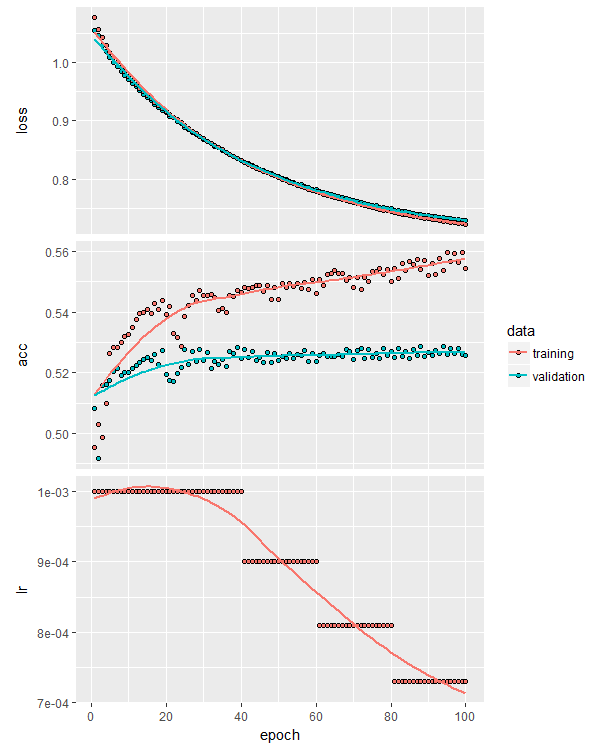
This particular training process resulted in an out of sample accuracy of 53.4%, slightly better than our original unregularized model. You can experiment with more or less regularization, as well as applying regularization to the bias terms and layer outputs.

Dropout

Dropout is another commonly used tool to fight overfitting. Whereas regularization is used throughout the machine learning ecosystem, dropout is specific to neural networks. Dropout is the random zeroing (“dropping out”) of some proportion of a layer’s outputs during training. The theory is that this helps prevents pairs or groups of nodes from learning random relationships that just happen to reduce the network loss on the training set (that is, result in overfitting).

Hinton and his colleagues, the discoverers of dropout, showed that it is generally superior to other forms of regularization and improves model performance on a variety of tasks. Read the original paper here.2As an aside, note the publication date of that paper: June 2014. That’s only about 3.5 years ago, yet dropout is already almost universally adopted throughout deep learning practice. This is a testament to just how quickly this field is evolving, and how closely integrated research and application really are.
Dropout is implemented in Keras as its own layer, layer_dropout(), which applies dropout on its inputs (that is, on the outputs of the previous layer in the stack). We need to supply the fraction of outputs to drop out, which we pass via the rate  parameter. In practice, dropout rates between 0.2 and 0.5 are common, but the optimal values for a particular problem and network configuration need to be determined through appropriate cross validation.
At the risk of getting ahead of ourselves, when applying dropout to recurrent architectures (which we’ll explore in a future post), we need to apply the same pattern of dropout at every timestep, otherwise dropout tends to hinder performance rather than enhance it.3If that statement makes no sense to you, ignore it for now. It will become clear when we get to recurrent networks in a future post. I wanted to include it here in case any readers start experimenting with recurrent networks before I get around to writing about them.
Here’s an example of how we build a feed-forward network with dropout in Keras:

###### FFN with dropout #####
model.drop <- keras_model_sequential()
model.drop %>%
  layer_dense(units = 150, activation = 'relu', input_shape = ncol(X_train)) %>%
  layer_dropout(rate = 0.3) %>%
  layer_dense(units = 150, activation = 'relu') %>%
  layer_dropout(rate = 0.3) %>%
  layer_dense(units = 150, activation = 'relu') %>%
  layer_dropout(rate = 0.3) %>%
  layer_dense(units = 1, activation = 'sigmoid')
summary(model.drop)
model.drop %>% compile(
  loss = 'binary_crossentropy',
  optimizer = optimizer_rmsprop(lr=0.001),
  metrics = c('accuracy')
)
filepath <- "C:/Users/Kris/Research/DeepLearningForTrading/model_drop.hdf5" # set up your own filepath
checkpoint <- callback_model_checkpoint(filepath = filepath, monitor = "val_acc", verbose = 1,
                                        save_best_only = TRUE,
                                        save_weights_only = FALSE, mode = "auto")
reduce_lr <- callback_reduce_lr_on_plateau(monitor = "val_acc", factor = 0.9,
                                           patience = 20, verbose = 1, mode = "auto",
                                           epsilon = 0.005, min_lr = 0.00001)
history.drop <- model.drop %>% fit(
  X_train, Y_train,
  epochs = 150, batch_size = nrow(X_train),
  validation_data = list(X_val, Y_val), shuffle = TRUE,
  callbacks = list(checkpoint, reduce_lr)
)
# plot training loss and accuracy
plot(history.drop)
max(history.drop$metrics$val_acc)
# load and evaluate best model
rm(model.drop)
model.drop <- keras:::keras$models$load_model(filepath)
model.drop %>% evaluate(X_test, Y_test)

Training the model using the same procedure as we used in the L2-regularized model above, including the reduce learning rate callback, we get the following training curves:
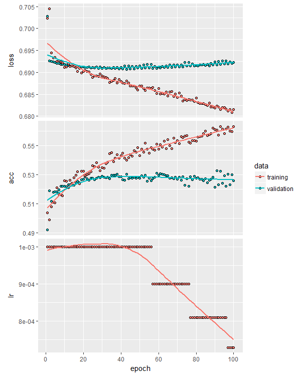One of the reasons dropout is so useful is that it enables the training of larger networks by reducing the likelihood of overfitting. Here’s the training curves for a similar model but this time eight layers deep:

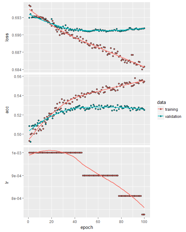
Notice that overfitting isn’t significantly worse than the shallower model. Also notice that it didn’t really learn any new, independent relationships from the data – this is evidenced by the failure to beat the previous model’s validation accuracy. Perhaps 53% is the upper out of sample accuracy limit for this data set and this approach to modeling it.
With dropout, you can also afford to use a larger learning rate, which means it is a good idea to make use of the reduce_lr_on_plateau  callback and kick off training with a higher learning rate, which can always be decayed as learning stalls.
Finally, one important consideration when using dropout is constraining the size of the network weights, particularly when a large learning rate is used early in training. In the Hinton et. al. paper linked above, constraining the weights was shown to improve performance in the presence of dropout.
Keras makes that easy thanks to the kernel_constraint  parameter of layer_dense() :

max_weight_constraint <- 5
model.drop <- keras_model_sequential()
model.drop %>%
  layer_dense(units = 150, activation = 'relu', kernel_constraint = constraint_maxnorm(max_value = max_weight_constraint), input_shape = ncol(X_train)) %>%
  layer_dropout(rate = 0.3) %>%
  layer_dense(units = 150, activation = 'relu', kernel_constraint = constraint_maxnorm(max_value = max_weight_constraint)) %>%
  layer_dropout(rate = 0.3) %>%
  layer_dense(units = 150, activation = 'relu', kernel_constraint = constraint_maxnorm(max_value = max_weight_constraint)) %>%
  layer_dropout(rate = 0.3) %>%
  layer_dense(units = 1, activation = 'sigmoid')

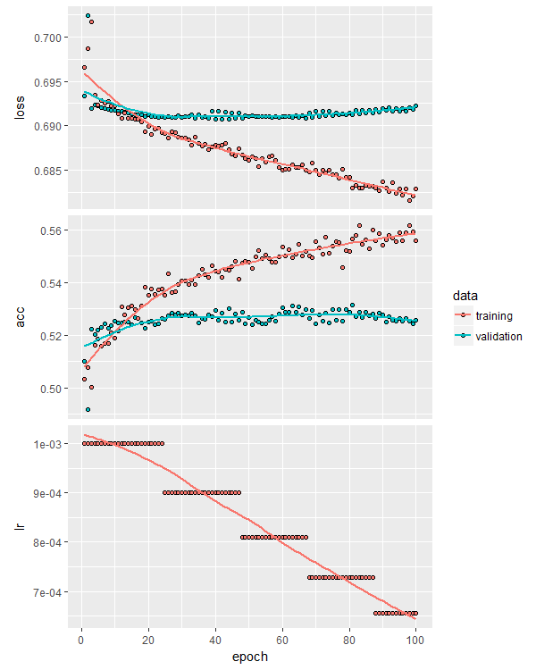
This model provided an ever-so-slight bump in validation accuracy:
And quite a stunning test-set equity curve:

# get predictions on test set and plot simple, frictionless PnL
preds <- model.drop %>% predict_proba(X_test)
threshold <- 0.5
trades <- ifelse(preds >= threshold, Y_test_raw, ifelse(preds <= 1-threshold, -Y_test_raw, 0))
plot(cumsum(trades), type='l')

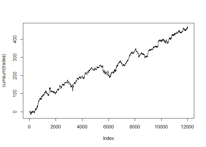
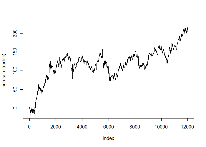
Interestingly, every experiment I performed in writing this post resulted in a positive out of sample equity curve. The results were all slightly different, even when using the same model setup, which reflects the non-deterministic nature of the training process (two identical networks trained on the same data can result in different weights, depending on the initial, pre-training weights of each network). Some equity curves were better than others, but they were all positive.
Here are some examples:

With L2-weight regularization and no dropout:

With a dropout rate of 0.2 applied at each layer, no regularization, and no weight constraints:

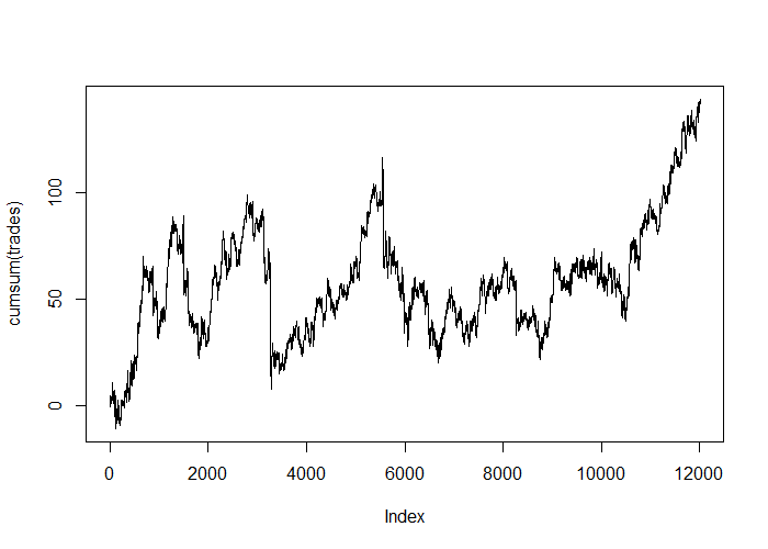
Of course, as mentioned in the last post, the edge of these models disappears when we apply retail spreads and broker commissions, but the frictionless equity curves demonstrate that deep learning, even using a simple feed-forward architecture, can extract predictive information from historical price action, at least for this particular data set, and that tools like regularization and dropout can make a difference to the quality of the model’s predictions.

Conclusions

This post demonstrated how to fight overfitting with regularization and dropout using Keras’ sequential model paradigm. While we further refined our previously identified slim edge in predicting the EUR/USD exchange rate’s direction, in practical terms, traders with access to retail spreads and commission will want to consider longer holding times to generate more profit per trade, or will need a more performant model to make money with this approach.

---

Where to from here?

• To find out why AI is taking off in finance, check out these insights from my days as an AI consultant to the finance industry 
• If this walk-through was useful for you, you might like to check out another how-to article on running trading algorithms on Google Cloud Platform
• If the technical details of neural networks are interesting for you, you might like our introductory article 
• Be sure to check out Part 1, Part 2, and Part 3 of this series on deep learning applications for trading. 
• If you’re ready to go deeper and get more practical tips and tricks on building robust trading systems, consider becoming a Robot Wealth Bootcamp member.