
This is the first post in a two-part series about the Hurst Exponent. Tom and I worked on this series together. I drew on some of his earlier work as well as other resources, including Quantstart.com.
UPDATE 03/01/16: The Python code below has been updated with a more accurate algorithm for calculating the Hurst Exponent.
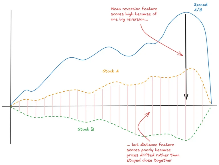
Mean-reverting time series have long attracted quantitative traders. Some of the biggest names in quant trading are said to have built their fortunes by exploiting mean reversion in financial data, particularly in constructed spreads used in pairs trading.
Naturally, identifying mean reversion is a key goal in algorithmic trading. However, this is harder than it seems, mainly due to the non-stationary nature of financial time series.
Ernie Chan’s Algorithmic Trading: Winning Strategies and Their Rationale is one of the better introductions to mean reversion. In his book, Ernie discusses several tools that help test whether a time series is mean-reverting. These include the Augmented Dickey-Fuller test and the Johansen test. We’ve explored both on Robot Wealth using simple R code [here] and [here].
Another tool for testing mean reversion is the Hurst Exponent.
What is the Hurst Exponent?
The Hurst Exponent, denoted H, helps characterize the behavior of a time series:
- H ≈ 0.5 → the series behaves like a random walk.
- H > 0.5 → the series trends, past movements are more likely to continue.
- H < 0.5 → the series is mean-reverting, tending to return to a long-term average.
However, working with Hurst can be tricky. It often yields unexpected results, and outcomes vary across different implementations. We also found that while various methods agree when applied to synthetic data, they diverge when tested on real financial time series.
Why Should Algo Traders Care?
This post introduces Python code for calculating the Hurst Exponent. In Part 2, we’ll dig deeper into how it works and discuss how to use it in practice.
Our goal is to demystify Hurst and show how to move beyond theory into something that can actually help in building trading strategies.
Hurst Exponent Python Implementation
Below is a simple Python script. It estimates the Hurst Exponent by plotting the relationship between lag and the standard deviation of lagged differences.
from numpy import *
from pylab import plot, show

# Create an arbitrary time series
ts = [0]
for i in range(1, 100000):
    ts.append(ts[i - 1] + random.randn())

# Compute standard deviations of differenced series for several lags
lags = range(2, 20)
tau = [sqrt(std(subtract(ts[lag:], ts[:-lag]))) for lag in lags]

# Plot on a log-log scale
plot(log(lags), log(tau))
show()

# Estimate Hurst Exponent as slope of the log-log plot
m = polyfit(log(lags), log(tau), 1)
hurst = m[0] * 2.0
print('hurst =', hurst)
In this code, we use lags from 2 to 20. These values are somewhat arbitrary but worked best when we tested them on synthetic data. Using larger lags tended to produce inaccurate results. Interestingly, this range matches the defaults in some standard implementations, such as MATLAB’s hurst function.
Next Steps and Practical Applications
In Part 2, we’ll explore how the choice of lags affects the Hurst calculation and show how tuning this parameter can lead to practical use in developing trading systems.
If you’ve used the Hurst Exponent, or any of the other mean reversion tests we mentioned, feel free to share your experiences in the comments. Thanks for reading!
Free Case Study:
A wantaway engineer’s journey into professional trading and out again
I went from engineering to an equity partnership at a prop trading firm to running my own systematic trading operation from home in Western Australia.
This case study is the full story – every mistake, every breakthrough, and some things I trade today.


Hi Kris,
I’ve had a brief look at Kaufman’s Efficiency Ratio. The results weren’t great, but I didn’t dig into it effectively enough to fully rule it out as a filter for the mean reversion systems I’m trading.
Happy to write it up with a proper analysis.
Nick
Hey Nick
I’d love to see a proper analysis of Kaufman’s Efficiency Ratio! You are welcome to share it here!
Cheers
Thanks Kris – will do – I’ll write it up and submit. Many thanks
Interesting post thanks… I’m currently investigating applying the Hurst exponent in machine learning to improve my trade selection. Try as I might, I can’t find a default Hurst Matlab function however!
Hi David,
I guess its not really a default function, but try this implementation of the generalized Hurst exponent:
https://au.mathworks.com/matlabcentral/fileexchange/30076-generalized-hurst-exponent?requestedDomain=www.mathworks.com
Thanks Kris, I’ll give that a try… I also stumbled across this new Matlab function gives 3 separate (!) estimates of the Hurst exponent too:
https://uk.mathworks.com/help/wavelet/ref/wfbmesti.html
Yes! This is a problem and one that we are going to attempt to get to the bottom of in the next post. Thanks for sharing that implementation.
Hi Kris,
Thanks for the article, incredibly interesting. I was just wondering if you could shed some light on where the sqrt of std comes from? I’ve been through both articles you linked to and find the RS method of calculating the Hurst exponent (the one originally derived by Hurst for the work on Nile levels) to be intuitively easier to understand. Looking at your update note, my guess would be that you were initially using that algorithm for calculating Hurst, but then moved on to the Generalized Hurst Exponent calculation that Mike from QuantStart uses on his page?
I’ve been through Mike’s explanation, but I still can’t seem to rationalize why we are using the square root of the standard deviation in this algorithm. Any light you could shed on that would be much appreciated.
Thanks again for the great article.
Hi Kris,
thanks for sharing.
I think we can save the sqrt() step here in : tau = [sqrt(std(subtract(ts[lag:], ts[:–lag]))) for lag in lags],
and no need to multiply 2 here in : hurst = m[0]*2.0.
So we the computation is simplified to:
…
tau = [std(subtract(ts[lag:], ts[:–lag])) for lag in lags],
…
hurst = m[0]
which saves computation and easier to be understood from the Hurst exponent definition.
But still thanks a lot for sharing this, learned a lot. 🙂
Regards
Andy
Nice one! Thanks Andy, that makes a lot of sense.
Hello,
Noob here, why are you taking the square root of the standard deviation of the differenced lags? Thought we were just trying to find the standard deviation?
Is it just so they are on a more condensed scale?
Hello,
Why do I get a low Hurst exponent with an only upward moving time series?
I get a hurst exponent of almost 0 when using the below generated time series (trends up by about 1).
for i in range(1,100000):
ts.append(i+1+random.uniform(0,1))