ETF Rotation Strategies in Zorro

At Robot Wealth we get more questions than even the most sleep-deprived trader can handle. So whilst we develop the algo equivalent of Siri and brag about how we managed to get 6 hours downtime last night, we thought we’d start a new format of blog posts — answering your most burning questions.
Lately our Class to Quant members have been looking to implement rotation-style ETF and equities strategies in Zorro, but just like your old high-school essays, starting is the biggest barrier. These types of strategies typically scan a universe of instruments and select one or more to hold until the subsequent rebalancing period. Zorro is my go-to choice for researching and even executing such strategies: its speed makes scanning even large universes of stocks quick and painless, and its scripting environment facilitates fast prototyping and iteration of the algorithm itself – once you’ve wrestled it for a while (get our free Zorro for Beginners video course here).
I’m going to walk you through a general design paradigm for constructing strategies like this with Zorro, and demonstrate the entire process with a simple rotation algorithm based on Gary Antonacci’s Dual Momentum. By the end you should have the skills needed to build a similar strategy yourself. Let’s begin!

ETF Rotation Strategy Design Paradigm

To construct a rotation style strategy in Zorro, we’d follow these general design steps:

1. Construct your universe of instruments by adding them to an assets list CSV file. There are examples in Zorro’s History folder, and I’ll put one together for you below.
2. Set up your rebalancing period using Zorro’s time and date functions.
3. Tell Zorro to reference the asset list you just created using the assetList  command.
4. Loop through each instrument in the list and perform whatever calculations or analysis your strategy requires for the selection of which instruments to hold.
5. Compare the results of the calculations/analysis performed in the prior step and construct the positions for the next period.

That’s pretty much it! Of course, the details of each step might differ slightly depending on the algorithm, and you will also need some position sizing and risk management, but in general, following these steps will get you 90% of the way there.
Not happy trading with a 90% complete strategy? No problem, let’s look at what this looks like in practice.

An Example

This example is based on Gary Antonacci’s Dual Momentum. We will simplify Gary’s slightly more nuanced version to the following: if US equities outperformed global equities and its return was positive, hold US equities. If global equities outperformed US equities and its return was positive, hold global equities. Otherwise, hold bonds.
Gary has done a mountain of research on Dual Momentum and found that it has outperformed for decades. In particular, it has tended to kick you out of equities during extended bear markets, while still getting you in for most of the bull markets. Check out Gary’s website for more information and consider getting hold of a copy of his book – you can read my review here.
Our simplified version of the strategy will use a universe of three ETFs that track US equities, global equities and short-term bonds. We will use the returns of these ETFs for both generation of our trading signals and actual trading (Gary’s approach is slightly more nuanced than that – again check out his website and book for more details).

Step 1: Construct our asset list

Our asset list contains the universe of instruments we wish to scan. In our case, we only need three ETFs. We’ll choose SPY for our US equities instrument, EFA for our global equities and SHY for our bonds ETF.
Zorro’s asset lists are CSV files that contain a bunch of parameters about the trading conditions of each instrument. This information is used in Zorro’s simulations, so it’s important to make it as accurate as possible. In many cases, Zorro can populate these files for us automatically by simply connecting to a broker, but in others, we need to do it manually (explained in our Zorro video course).
Our asset list for this strategy will look like this:

Name,Price,Spread,RollLong,RollShort,PIP,PIPCost,MarginCost,Leverage,LotAmount,Commission,Symbol
SPY,269.02,0.1,0,0,0.01,0.01,0,1,1,0.02,
SHY,83.61,0.1,0,0,0.01,0.01,0,1,1,0.02,
EFA,69.44,0.1,0,0,0.01,0.01,0,1,1,0.02,

You can see that most of the parameters are actually the same for each instrument, so we can use copy and paste to make the construction of this file less tedious than it would otherwise be. For other examples of such files, just look in Zorro’s History folder.
Save this file as a CSV file called AssetsDM.csv and place it in your History folder (which is where Zorro will go looking for it shortly).

Step 2: Set up rebalance period

Here we are going to rebalance our portfolio every month. We decided to avoid the precise start/end of the month and rebalance on the third trading day of the month. You can experiment with this parameter to get a feel for how much it affects the strategy.
Simply wrap the trading logic in the following if()  statement:

if(tdm() == 3)
{
...
}

Step 3: Tell Zorro about your new asset list

In the initial run of the script, we want Zorro to reference the newly created asset list. Also, if we don’t have data for these instruments, we want to download it in the initial run. We’ll use Alpha Vantage end-of-day data, which can be accessed directly from within Zorro scripts. These lines of code take care of that for us:

if(is(INITRUN))
    {
        assetList("History\\AssetsDM.csv");
        string Name;
        while(Name = loop(Assets))
        {
            assetHistory(Name, FROM_AV);
        }
    }

Note that this assumes you’ve entered your Alpha Vantage API key in the Zorro.ini or ZorroFix.ini configuration files, which live in Zorro’s base directory. If you don’t have an Alpha Vantage API key head over to the Alpha Vantage website to claim one.

Step 4: Loop through instruments and perform calculations

For our dual momentum strategy, we need to know the return of each instrument over the portfolio formation period. So we can loop through each asset in our list, calculate the return, and store it in an array for later use.
If you intend on using Zorro’s optimizer, perform the loop operation using a construct like:

for(i=0; Name=Assets[i]; i++)
{
...
}

If you don’t intend on using the optimizer, you can safely use the more convenient while(loop(Assets))  construct.
The reason we don’t use the latter in an optimization run is that the loop()  function is handled differently in Zorro’s Train mode, and will actually run a separate simulation for each instrument in the loop. This is perfect in the instance we want to trade a particular algorithm across multiple, known instruments – something like a moving average crossover traded on each stock in the S&P500, where we wanted to optimize the moving average periods separately for each instrument1Not that I would recommend such a strategy of course!. But in an algorithm that compares and selects instruments from a universe of instruments, optimizing some parameter set on each one individually wouldn’t make sense.
This is actually a really common mistake when developing these type of strategies in Zorro, but if you understand the behavior of loop()  in Zorro’s Train mode, it’s one that you probably won’t make again.
Here’s the code for performing the looped return calculations:

if(tdm()==3)
    {
        asset_num = 0;
        while(loop(Assets))
        {
            asset(Loop1);
            Returns[asset_num] = (priceClose(0)-priceClose(DAYS))/priceClose(DAYS);
            asset_num++;
        }
    ...

Step 5 Compare the results and construct the positions for the next period.

Recalling our dual momentum trading logic, we firstly check if US equities outperformed global equities. If so, we then check that their absolute return was positive. If so, then we hold US equities. If global bonds outperformed US equities, we check that their absolute return was positive. If so, then we hold global equities. If neither US equities nor global equities had a positive return, we hold bonds.
If you stop and think about that logic, we are really just holding the instrument with the highest return in the formation period, with the added condition that for the equities instruments, they also had a positive absolute return. We could implement that trading logic like so:

// sort returns lowest to highest
int* idx = sortIdx(Returns, asset_num);
// exit any positions where asset is ranked in bottom 2 and is not bonds
int i;
for(i=0;i<2;i++)
{
    asset(Assets[idx[i]]);
    if(Asset != "SHY")
    {
        if(NumOpenLong > 0)
        {
            printf("\nAsset to close: %s", Asset);
            exitLong();
        }
    }
}
// asset to hold
asset(Assets[idx[2]]);
/*
check if asset is bonds, if so buy
if not, if return of highest ranked asset is positive, buy
otherwise, switch to bonds and buy
*/
if(Asset == "SHY")
{
    // don't apply time series momentum to bonds
    enterLong();
}
else if(Returns[idx[2]] > 0) //time-series momentum condition
{
    enterLong();
    asset("SHY");
    exitLong();
}
else
{
    // switch to bonds and buy
    asset("SHY");
    enterLong();
}
}

This is probably the most confusing part of the script, so let’s talk about it in some detail. Firstly, the line

int* idx = sortIdx(Returns, asset_num)

returns an array of the indexes of the Returns  array, sorted from lowest to highest. Say our Returns  array held the numbers 4, -2, 2. Our array idx  would contain 1, 2, 0 because the item at Returns[1]  is the lowest number, followed by the number at Returns[2] , with Returns[0]  being the highest number. This might seem confusing, but it will provide us with a convenient way to access the highest ranked instrument directly from the Assets array, which holds the names of the instruments in the order called by our loop()  function.
In lines 5-17, we firstly use this feature to exit any open positions that aren’t the highest ranked asset – provided those lower ranked assets aren’t bonds. Remember, we might want to hold a bond position, even if it isn’t the highest ranked asset. So we won’t exit any open bond positions just yet.
Next, in line 20, we switch the highest ranked instrument. If that instrument is bonds, we don’t bother checking the absolute return condition (it doesn’t apply to bonds) and go long. If that instrument is one of the equities ETFs, we check the absolute return condition. If that turns out to be true, we enter a long position in that ETF, then switch to bonds and exit any open position we may have been holding.
Finally, if the absolute return condition on our top-ranked equities ETFs wasn’t true, we switch to bonds and enter a long position.

Position Sizing

In this case we are simply going to be fully invested with all of our starting capital and any accrued profits in the currently selected instrument. Here’s the code for accomplishing that:

Capital = 10000;
Margin = Capital+WinTotal-LossTotal;

Note that this is only possible because we are trading these instruments with no leverage (leverage is defined in the asset list above). If we were using leverage, we’d obviously have to reduce the amount of margin invested in a given position.

Putting it all Together

Finally, here’s the complete code listing for our simple Dual Momentum algorithm. In order for the script to run, remember to save a copy of the asset list in Zorro’s History folder, and enter your Alpha Vantage API key in the Zorro.ini or ZorroFix.ini configuration files.

/*
Dual momentum in Zorro
*/
#define NUM_ASSETS 3
#define DAYS 252
int asset_num;
function run()
{
    set(PLOTNOW);
    PlotWidth = 1200;
    StartDate = 20040101;
    EndDate = 20170630;
    BarPeriod = 1440;
    LookBack = DAYS;
    MaxLong = 1;
    if(is(INITRUN))
    {
        assetList("History\\AssetsDM.csv");
        string Name;
        while(Name = loop(Assets))
        {
            assetHistory(Name, FROM_AV);
        }
    }
    var Returns[NUM_ASSETS];
    int position_diff;
    if(tdm()==3)
    {
        asset_num = 0;
        while(loop(Assets))
        {
            asset(Loop1);
            Returns[asset_num] = (priceClose(0)-priceClose(DAYS))/priceClose(DAYS);
            asset_num++;
        }
        Capital = 10000;
        Margin = Capital+WinTotal-LossTotal;
        // sort returns lowest to highest
        int* idx = sortIdx(Returns, asset_num);
        // exit any positions where asset is ranked in bottom 2 and is not bonds
        int i;
        for(i=0;i<2;i++)
        {
            asset(Assets[idx[i]]);
            if(Asset != "SHY")
            {
                if(NumOpenLong > 0)
                {
                    printf("\nAsset to close: %s", Asset);
                    exitLong();
                }
            }
        }
        // asset to hold
        asset(Assets[idx[2]]);
        /*
        check if asset is bonds, if so buy
        if not, if return of highest ranked asset is positive, buy
        otherwise, switch to bonds and buy
        */
        if(Asset == "SHY")
        {
            // don't apply time series momentum to bonds
            enterLong();
        }
        else if(Returns[idx[2]] > 0) //time-series momentum condition
        {
            enterLong();
            asset("SHY");
            exitLong();
        }
        else
        {
            // switch to bonds and buy
            asset("SHY");
            enterLong();
        }
    }
}

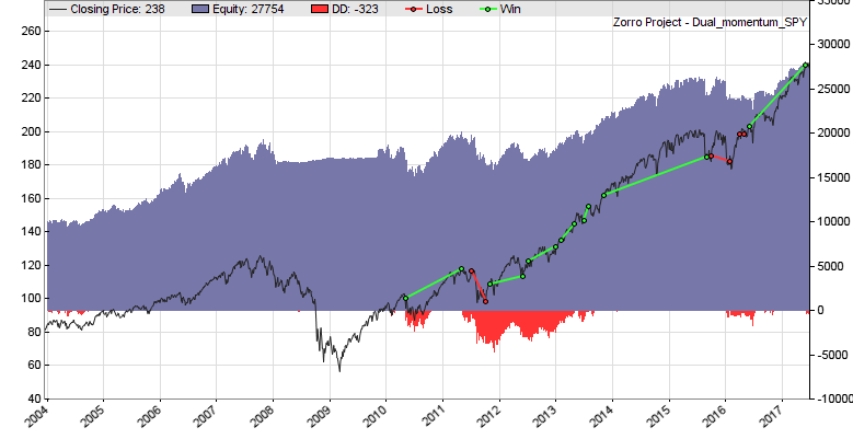
Over the simulation period, the strategy returns a Sharpe Ratio of 0.52. That’s pretty healthy for something that trades so infrequently. In terms of gross returns, the starting capital of $10,000 was almost tripled, and the maximum drawdown was approximately $4,700. One of the main limitations of the strategy is that by design, it is highly concentrated, taking only single position at a time.
Here’s the equity curve:

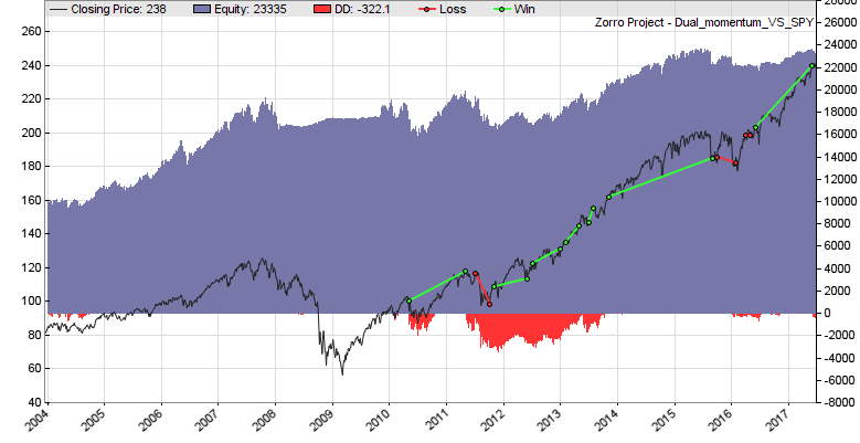
However, being fully invested at all times may not be the smartest way to construct a portfolio. A more thoughtful approach to position sizing and careful use of leverage, as we teach inside the Robot Wealth community, can yield better risk-adjusted returns. For example, something like this gives a similar return, while the maximum drawdown is reduced by around 25%:

Robot Wealth Members can access the script that produced these results via the Strategies and Tools section of their dashboard.

Conclusion

Rotation style strategies* require a slightly different design approach than strategies for whom the tradable subset of instruments is static. By following the five broad design principles described here, you can leverage Zorro’s speed, power and flexibility to develop these types of strategies. Good luck and happy profits!
*This is just one of the many algorithmic trading fundamentals we cover inside Class to Quant. Not only are our members improving their trading performance with our beginner to advanced courses, but together they’re building functioning strategies inside our community as part of our Algo Laboratory projects. If you’re interested and want to find out more, try Class to Quant for 30 days risk free. I’d love to meet you inside.

Where to from here?

• Check out my review of Gary Antonacci’s Dual Momentum, and explore some other variations written in R
  
• Get our free Zorro for Beginners video series, and go from beginner to Zorro trader in just 90 minutes
• If you’re ready to go deeper and get more practical tips and tricks on building robust trading systems, as well as joining our strong community of traders, check out our flagship offer Class to Quant.