
If you’re interested in using artificial neural networks (ANNs) for algorithmic trading, but don’t know where to start, then this article is for you. Normally if you want to learn about neural networks, you need to be reasonably well versed in matrix and vector operations – the world of linear algebra. This article is different. I’ve attempted to provide a starting point that doesn’t involve any linear algebra and have deliberately left out all references to vectors and matrices. If you’re not strong on linear algebra, but are curious about neural networks, then I think you’ll enjoy this introduction. In addition, if you decide to take your study of neural networks further, when you do inevitably start using linear algebra, it will probably make a lot more sense as you’ll have something of head start. The best place to start learning about neural networks is the perceptron. The perceptron is the simplest possible artificial neural network, consisting of just a single neuron and capable of learning a certain class of binary classification problems.1 Perceptrons are the perfect introduction to ANNs and if you can understand how they work, the leap to more complex networks and their attendant issues will not be nearly as far. So we will explore their history, what they do, how they learn, where they fail. We’ll build our own perceptron from scratch and train it to perform different classification tasks which will provide insight into where they can perform well, and where they are hopelessly outgunned. Lastly, we’ll explore one way we might apply a perceptron in a trading system.2
A Brief History of the Perceptron
The perceptron has a long history, dating back to at least the mid 1950s. Following its discovery, the New York Times ran an article that claimed that the perceptron was the basis of an artificial intelligence (AI) that would be able to walk, talk, see and even demonstrate consciousness. Soon after, this was proven to be hyperbole on a staggering scale, when the perceptron was shown to be wholly incapable of classifying certain types of problems. The disillusionment that followed essentially led to the first AI winter, and since then we have seen a repeating pattern of hyperbole followed by disappointment in relation to artificial intelligence.3 Still, the perceptron remains a useful tool for some classification problems and is the perfect place to start if you’re interested in learning more about neural networks. Before we demonstrate it in a trading application, let’s find out a little more about it.Artificial Neural Networks: Modelling Nature
Algorithms modelled on biology are a fascinating area of computer science. Undoubtedly you’ve heard of the genetic algorithm, which is a powerful optimization tool modelled on evolutionary processes. Nature has been used as a model for other optimization algorithms, as well as the basis for various design innovations. In this same vein, ANNs attempt to learn relationships and patterns using a somewhat loose model of neurons in the brain. The perceptron is a model of a single neuron.4 In an ANN, neurons receive a number of inputs, weight each of those inputs, sum the weights, and then transform that sum using a special function called an activation function, of which there are many possible types. The output of that activation function is then either used as the prediction (in a single neuron model) or is combined with the outputs of other neurons for further use in more complex models, which we’ll get to in another article. Here’s a sketch of that process in an ANN consisting of a single neuron: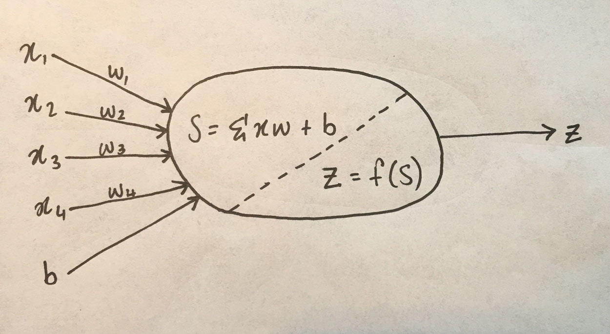 Here, (x_1, x_2, etc) are the inputs. (b) is called the bias term, think of it like the intercept term in a linear model (y = mx + b). (w_1, w_2, etc) are the weights applied to each input. The neuron firstly sums the weighted inputs (and the bias term), represented by (S) in the sketch above. Then, (S) is passed to the activation function, which simply transforms (S) in some way. The output of the activation function, (z) is then the output of the neuron.
The idea behind ANNs is that by selecting good values for the weight parameters (and the bias), the ANN can model the relationships between the inputs and some target. In the sketch above, (z) is the ANN’s prediction of the target given the input variables.
In the sketch, we have a single neuron with four weights and a bias parameter to learn. It isn’t uncommon for modern neural networks to consist of hundreds of neurons across multiple layers, where the output of each neuron in one layer is input to all the neurons in the next layer. Such a fully connected network architecture can easily result in many thousands of weight parameters. This enables ANNs to approximate any arbitrary function, linear or nonlinear.
The perceptron consists of just a single neuron, like in our sketch above. This greatly simplifies the problem of learning the best weights, but it also has implications for the class of problems that a perceptron can solve.
Here, (x_1, x_2, etc) are the inputs. (b) is called the bias term, think of it like the intercept term in a linear model (y = mx + b). (w_1, w_2, etc) are the weights applied to each input. The neuron firstly sums the weighted inputs (and the bias term), represented by (S) in the sketch above. Then, (S) is passed to the activation function, which simply transforms (S) in some way. The output of the activation function, (z) is then the output of the neuron.
The idea behind ANNs is that by selecting good values for the weight parameters (and the bias), the ANN can model the relationships between the inputs and some target. In the sketch above, (z) is the ANN’s prediction of the target given the input variables.
In the sketch, we have a single neuron with four weights and a bias parameter to learn. It isn’t uncommon for modern neural networks to consist of hundreds of neurons across multiple layers, where the output of each neuron in one layer is input to all the neurons in the next layer. Such a fully connected network architecture can easily result in many thousands of weight parameters. This enables ANNs to approximate any arbitrary function, linear or nonlinear.
The perceptron consists of just a single neuron, like in our sketch above. This greatly simplifies the problem of learning the best weights, but it also has implications for the class of problems that a perceptron can solve.
What’s an Activation Function?
The purpose of the activation function is to take the input signal (that’s the weighted sum of the inputs and the bias) and turn it into an output signal. There are many different activation functions that convert an input signal in a slightly different way, depending on the purpose of the neuron. Recall that the perceptron is a binary classifier. That is, it predicts either one or zero, on or off, up or down, etc. It follows then that our activation function needs to convert the input signal (which can be any real-valued number) into either a one or a zero5corresponding to the predicted class. In biological terms, think of this activation function as firing (activating) the neuron (telling it to pass the signal on to the next neuron) when it returns 1, and doing nothing when it returns 0. What sort of function accomplishes this? It’s called a step function, and its mathematical expression looks like this: [f(z) =\begin{cases} 1, & \text{if $z$ > 0} \ 0, & \text{otherwise} \end{cases}] And when plotted, it looks like this: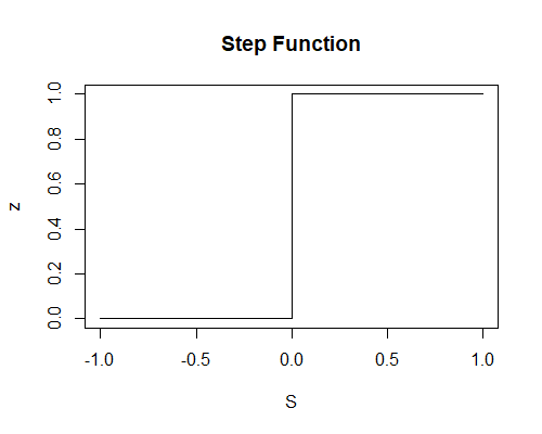 This function then transforms any weighted sum of the inputs (S) and converts it into a binary output (either 1 or 0). The trick to making this useful is finding (learning) a set of weights, (w), that lead to good predictions using this activation function.
How Does a Perceptron Learn?
We already know that the inputs to a neuron get multiplied by some weight value particular to each individual input. The sum of these weighted inputs is then transformed into an output via an activation function. In order to find the best values for our weights, we start by assigning them random values and then start feeding observations from our training data to the perceptron, one by one. Each output of the perceptron is compared with the actual target value for that observation, and, if the prediction was incorrect, the weights adjusted so that the prediction would have been closer to the actual target. This is repeated until the weights converge. In perceptron learning, the weight update function is simple: when a target is misclassified, we simply take the sign of the error and then add or subtract the inputs that led to the misclassifiction to the existing weights. If that target was -1 and we predicted 1, the error is (-1 -1 = -2). We would then subtract each input value from the current weights (that is, (w_i = w_i – x_i)). If the target was 1 and we predicted -1, the error is (1 – -1 = 2), so then add the inputs to the current weights (that is, (w_i = w_i + x_i)).6 This has the effect of moving the classifier’s decision boundary (which we will see below) in the direction that would have helped it classify the last observation correctly. In this way, weights are gradually updated until they converge. Sometimes (in fact, often) we’ll need to iterate through each of our training observations more than once in order to get the weights to converge. Each sweep through the training data is called an epoch.Implementing a Perceptron from Scratch
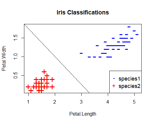
Next, we’ll code our own perceptron learning algorithm from scratch using R. We’ll train it to classify a subset of the iris data set.7 In the full iris data set, there are three species. However, perceptrons are for binary classification (that is, for distinguishing between two possible outcomes). Therefore, for the purpose of this exercise, we remove all observations of one of the species (here, virginica), and train a perceptron to distinguish between the remaining two. We also need to convert the species classification into a binary variable: here we use 1 for the first species, and -1 for the other. Further, there are four variables in addition to the species classification: petal length, petal width, sepal length and sepal width. For the purposes of illustration, we’ll train our perceptron using only petal length and width and drop the other two measurements. These data transformations result in the following plot of the remaining two species in the two-dimensional feature space of petal length and petal width: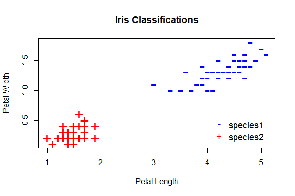 The plot suggests that petal length and petal width are strong predictors of species – at least in our training data set. Can a perceptron learn to tell them apart?
Training our perceptron is simply a matter of initializing the weights (here we initialize them to zero) and then implementing the perceptron learning rule, which just updates the weights based on the error of each observation with the current weights. We do that in a for() loop which iterates over each observation, making a prediction based on the values of petal length and petal width of each observation, calculating the error of that prediction and then updating the weights accordingly.
In this example we perform five sweeps through the entire data set, that is, we train the perceptron for five epochs. At the end of each epoch, we calculate the total number of misclassified training observations, which we hope will decrease as training progresses. Here’s the code:
The plot suggests that petal length and petal width are strong predictors of species – at least in our training data set. Can a perceptron learn to tell them apart?
Training our perceptron is simply a matter of initializing the weights (here we initialize them to zero) and then implementing the perceptron learning rule, which just updates the weights based on the error of each observation with the current weights. We do that in a for() loop which iterates over each observation, making a prediction based on the values of petal length and petal width of each observation, calculating the error of that prediction and then updating the weights accordingly.
In this example we perform five sweeps through the entire data set, that is, we train the perceptron for five epochs. At the end of each epoch, we calculate the total number of misclassified training observations, which we hope will decrease as training progresses. Here’s the code:
# perceptron initial weights
w1 = 0
w2 = 0
b = 0
# perceptron learning
epochs <- 5
errors <- vector()
for(j in c(1:epochs))
{
  for(i in c(1:nrow(iris)))
  {
    yhat <- ifelse(w1*iris$Petal.Length[i] + w2*iris$Petal.Width[i] + b > 0, 1, -1) #prediction of current observation
    error = iris$Species[i] - yhat #will be either 0, 2 or -2
    w1 <- w1 + error*iris$Petal.Length[i]
    w2 <- w2 + error*iris$Petal.Width[i]
    b <- b + error
  }
  # end of epoch
  preds <- ifelse(w1*iris$Petal.Length + w2*iris$Petal.Width + b > 0, 1, -1) #predict on whole training set
  errors[j] <- sum(abs(iris$Species - preds))/2 # calculate errors
}
plot(c(1:epochs), errors, type='l', xlab='epoch') # plot error rate at each epoch
Here’s the plot of the error rate:
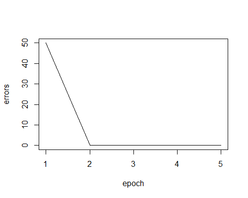 We can see that it took two epochs to train the perceptron to correctly classify the entire dataset. After the first epoch, the weights hadn’t been sufficiently updated. In fact, after epoch 1, the perceptron predicted the same class for every observation! Therefore it misclassified 50 out of the 100 observations (there are 50 observations of each species in the data set). However after two epochs, the perceptron was able to correctly classify the entire data set by learning appropriate weights.
Another, perhaps more intuitive way, to view the weights that the perceptron learns is in terms of its decision boundary. In geometric terms, for the two-dimensional feature space in this example, the decision boundary is the a straight line separating the perceptron’s predictions. On one side of the line, the perceptron always predicts -1, and on the other, it always predicts 1.8
We can derive the decision boundary from the perceptron’s activation function:
[f(z) =\begin{cases} 1, & \text{if $z$ > 0} \ 0, & \text{otherwise} \end{cases}]
where (z = w_1x_1 + w_2x_2 + b)
The decision boundary is simply the line that defines the location of the step in the activation function. That step occurs at (z=0), so our decision boundary is given by
[w_1x_1 + w_2x_2 + b\ = 0 ]
Equivalently [x_2 = -\frac{w_1}{w_2}x_1 – \frac{b}{w_2}]
which defines a straight line in (x_1, x_2) feature space.
In our iris example, the perceptron learned the following decision boundary:
We can see that it took two epochs to train the perceptron to correctly classify the entire dataset. After the first epoch, the weights hadn’t been sufficiently updated. In fact, after epoch 1, the perceptron predicted the same class for every observation! Therefore it misclassified 50 out of the 100 observations (there are 50 observations of each species in the data set). However after two epochs, the perceptron was able to correctly classify the entire data set by learning appropriate weights.
Another, perhaps more intuitive way, to view the weights that the perceptron learns is in terms of its decision boundary. In geometric terms, for the two-dimensional feature space in this example, the decision boundary is the a straight line separating the perceptron’s predictions. On one side of the line, the perceptron always predicts -1, and on the other, it always predicts 1.8
We can derive the decision boundary from the perceptron’s activation function:
[f(z) =\begin{cases} 1, & \text{if $z$ > 0} \ 0, & \text{otherwise} \end{cases}]
where (z = w_1x_1 + w_2x_2 + b)
The decision boundary is simply the line that defines the location of the step in the activation function. That step occurs at (z=0), so our decision boundary is given by
[w_1x_1 + w_2x_2 + b\ = 0 ]
Equivalently [x_2 = -\frac{w_1}{w_2}x_1 – \frac{b}{w_2}]
which defines a straight line in (x_1, x_2) feature space.
In our iris example, the perceptron learned the following decision boundary:
 Here’s the complete code for training this perceptron and producing the plots shown above:
### PERCEPTRON FROM SCRATCH ####
# load data
data(iris)
# transform data to binary classification problem using two inputs
iris <- iris[iris$Species != 'virginica', c('Petal.Length', 'Petal.Width', 'Species')]
iris$Species <- ifelse(iris$Species=='versicolor', 1, -1)
# plot data
plot(iris[, c(1,2)],pch=ifelse(iris$Species>0,"-","+"),
     col=ifelse(iris$Species>0,"blue","red"), cex=2,
     main = 'Iris Classifications')
legend("bottomright", c("species1", "species2"), col=c("blue", "red"), pch=c("-","+"), cex=1.1)
# perceptron initial weights
w1 = 0
w2 = 0
b = 0
# perceptron learning
epochs <- 5
errors <- vector()
for(j in c(1:epochs))
{
  for(i in c(1:nrow(iris)))
  {
    yhat <- ifelse(w1*iris$Petal.Length[i] + w2*iris$Petal.Width[i] + b > 0, 1, -1)
    error = iris$Species[i] - yhat #will be either 0, 2 or -2
    w1 <- w1 + error*iris$Petal.Length[i]
    w2 <- w2 + error*iris$Petal.Width[i]
    b <- b + error
  }
  # end of epoch
  preds <- ifelse(w1*iris$Petal.Length + w2*iris$Petal.Width + b > 0, 1, -1)
  errors[j] <- sum(abs(iris$Species - preds))/2
}
slope <- -w1/w2
intercept <- -b/w2
abline(intercept, slope)
plot(c(1:epochs), errors, type='l', xlab='epoch')
Congratulations! You just built and trained your first neural network.
Let’s now ask our perceptron to learn a slightly more difficult problem. Using the same iris data set, this time we remove the setosa species and train a perceptron to classify virginica and versicolor on the basis of their petal lengths and petal widths. When we plot these species in their feature space, we get this:
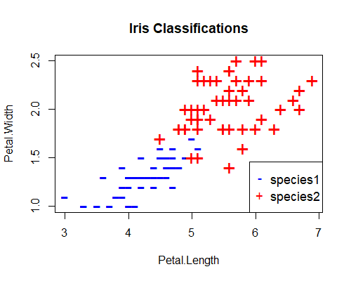 This looks a slightly more difficult problem, as this time the difference between the two classifications is not as clear cut. Let’s see how our perceptron performs on this data set.
This time, we introduce the concept of the learning rate, which is important to understand if you decide to pursue neural networks beyond the perceptron. The learning rate controls the speed with which weights are adjusted during training. We simply scale the adjustment by the learning rate: a high learning rate means that weights are subject to bigger adjustments. Sometimes this is a good thing, for example when the weights are far from their optimal values. But sometimes this can cause the weights to oscillate back and forth between two high-error states without ever finding a better solution. In that case, a smaller learning rate is desirable, which can be thought of as fine tuning of the weights.
Finding the best learning rate is largely a trial and error process, but a useful approach is to reduce the learning rate as training proceeds. In the example below, we do that by scaling the learning rate by the inverse of the epoch number.
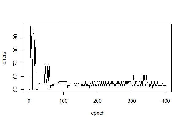
Here’s a plot of our error rate after training in this manner for 400 epochs:
This looks a slightly more difficult problem, as this time the difference between the two classifications is not as clear cut. Let’s see how our perceptron performs on this data set.
This time, we introduce the concept of the learning rate, which is important to understand if you decide to pursue neural networks beyond the perceptron. The learning rate controls the speed with which weights are adjusted during training. We simply scale the adjustment by the learning rate: a high learning rate means that weights are subject to bigger adjustments. Sometimes this is a good thing, for example when the weights are far from their optimal values. But sometimes this can cause the weights to oscillate back and forth between two high-error states without ever finding a better solution. In that case, a smaller learning rate is desirable, which can be thought of as fine tuning of the weights.
Finding the best learning rate is largely a trial and error process, but a useful approach is to reduce the learning rate as training proceeds. In the example below, we do that by scaling the learning rate by the inverse of the epoch number.
Here’s a plot of our error rate after training in this manner for 400 epochs:
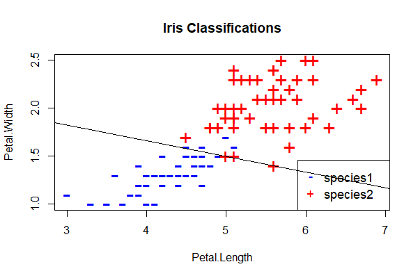
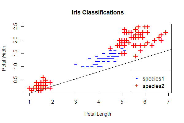
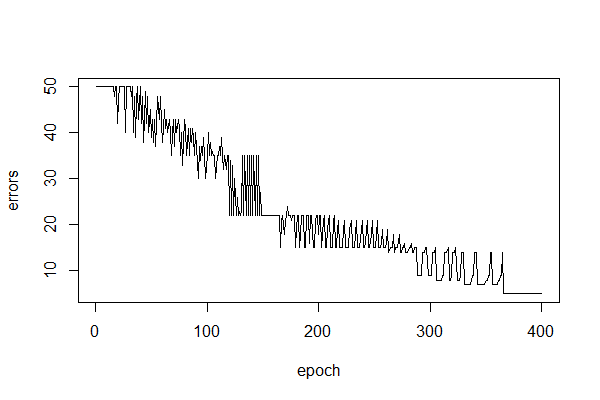 You can see that training proceeds much less smoothly and takes a lot longer than last time, which is a consequence of the classification problem being more difficult. Also note that the error rate is never reduced to zero, that is, the perceptron is never able to perfectly classify this data set. Here’s a plot of the decision boundary, which demonstrates where the perceptron makes the wrong predictions:
 Here’s the code for this perceptron:
# load data
data(iris)
# transform data to binary classification problem using two inputs
iris <- iris[iris$Species != 'setosa', c('Petal.Length', 'Petal.Width', 'Species')]
iris$Species <- ifelse(iris$Species=='versicolor', 1, -1)
# plot data
plot(iris[, c(1,2)],pch=ifelse(iris$Species>0,"-","+"),
     col=ifelse(iris$Species>0,"blue","red"), cex=2,
     main = 'Iris Classifications')
legend("bottomright", c("species1", "species2"), col=c("blue", "red"), pch=c("-","+"), cex=1.1)
# perceptron initial weights
w1 = 0
w2 = 0
b = 0
# perceptron learning
epochs <- 400
errors <- vector()
for(j in c(1:epochs))
{
  learn.rate <- 1/j # set learning rate
  for(i in c(1:nrow(iris)))
  {
    yhat <- ifelse(w1*iris$Petal.Length[i] + w2*iris$Petal.Width[i] + b > 0, 1, -1)
    error = iris$Species[i] - yhat #will be either 0, 2 or -2
    w1 <- w1 + learn.rate*error*iris$Petal.Length[i]
    w2 <- w2 + learn.rate*error*iris$Petal.Width[i]
    b <- b + learn.rate*error
  }
  # end of epoch
  preds <- ifelse(w1*iris$Petal.Length + w2*iris$Petal.Width + b > 0, 1, -1)
  errors[j] <- sum(abs(iris$Species - preds))/2
}
slope <- -w1/w2
intercept <- -b/w2
abline(intercept, slope)
plot(c(1:epochs), errors, type='l', xlab='epoch')
Where Do Perceptrons Fail?
In the first example above, we saw that our versicolor and setosa iris species could be perfectly separated by a straight line (the decision boundary) in their feature space. Such a classification problem is said to be linearly separable and (spoiler alert) is where perceptrons excel. In the second example, we saw that versicolor and virginica were almost linearly separable, and our perceptron did a reasonable job, but could never perfectly classify the whole data set. In this next example, we’ll see how they perform on a problem that isn’t linearly separable at all. Using the same iris data set, this time we classify our iris species as either versicolor or other (that is setosa and virginica get the same classification) on the basis of their petal lengths and petal widths. When we plot these species in their feature space, we get this: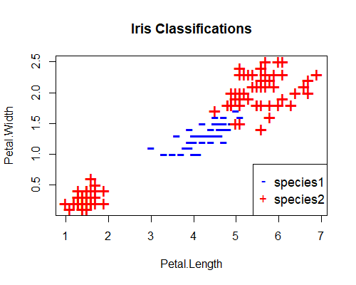 This time, there is no straight line that can perfectly separate the two species. Let’s see how our perceptron performs now. Here’s the error rate over 400 epochs and the decision boundary:
 We can see that the perceptron fails to distinguish between the two classes. This is typical of the performance of the perceptron on any problem that isn’t linearly separable. Hence my comment at the start of this unit (see footnote 2) that I’m skeptical that perceptrons can find practical application in trading. Maybe you can find a use case in trading, but even if not, they provide an excellent foundation for exploring more complex networks which can model more complex relationships.
A Perceptron Implementation for Algorithmic Trading
The Zorro trading automation platform includes a flexible perceptron implementation. If you haven’t heard of Zorro, it is a fast, accurate and powerful backtesting/execution platform that abstracts a lot of tedious programming tasks so that the user is empowered to concentrate on efficient research. It uses a simple C-based scripting language that takes almost no time to learn if you already know C, and a week or two if you don’t (although of course mastery can take much longer). This makes it an excellent choice for independent traders and those getting started with algorithmic trading. While the software sacrifices little for the abstraction that enables efficient research, experienced quant developers or those with an abundance of spare time might take issue with that aspect of the software, as it’s not open source, so it isn’t for everyone. But it’s a great choice for beginners and DIY traders who maintain a day job. If you want to learn to use Zorro, even if you’re not a programmer, we can help. Zorro’s perceptron implementation allows us to define any features we think are pertinent, and to specify any target we like, which Zorro automatically converts it to a binary variable (by default, positive values are given one class; negative values the other). After training, Zorro’s perceptron predicts either a positive or negative value corresponding to the positive and negative classes respectively. Here’s the Zorro code for implementing a perceptron that tries to predict whether the 5-day price change in the EUR/USD exchange rate will be greater than 200 pips, based on recent returns and volatility, whose predictions are tested under a walk-forward framework:/* PERCEPTRON
*/
function run()
{
set(RULES|PEEK|PLOTNOW|OPENEND);
StartDate = 20100101;
EndDate = 20161231;
BarPeriod = 1440;
LookBack = 100;
BarZone = WET;
BarOffset = 9*60;
asset("EUR/USD");
if(Train) Hedge = 2; //needed for training trade results
// set up walk-forward parameters
int TST = 50*1440/BarPeriod; //number of bars in test period
int TRN = 500*1440/BarPeriod; //number of bars in training period
DataSplit = 100*TRN/(TST+TRN);
WFOPeriod = TST+TRN;
//data
vars Close = series(priceClose());
//signals
var Sig1 = scale(ATR(10)-ATR(50), 100);
var Sig2 = (Close[0]-Close[1])/Close[1];
var Sig3 = (Close[0]-Close[5])/Close[5];
var Sig4 = (Close[0]-Close[10])/Close[10];
var ObjLong;
var ObjShort;
if(priceClose(-5) - priceClose(0) > 200*PIP) ObjLong = 1;
else ObjLong = -1;
if(priceClose(-5) - priceClose(0) < -200*PIP) ObjShort = 1;
else ObjShort = -1;
LifeTime = 5;
var l = adviseLong(PERCEPTRON+BALANCED, ObjLong, Sig1, Sig2, Sig3, Sig4);
var s = adviseShort(PERCEPTRON+BALANCED, ObjShort, Sig1, Sig2, Sig3, Sig4);
if(!Train)
{
if(l > 0 and s < 0) reverseLong(1);
else if(s > 0 and l < 0) reverseShort(1);
}
plot("l", l, NEW, GREEN);
plot("s", s, NEW, RED);
}
Zorro firstly outputs a trained perceptron for predicting long and short 5-day price moves greater than 200 pips for each walk-forward period, and then tests their out-of-sample predictions.
Here’s the walk-forward equity curve of our example perceptron trading strategy:
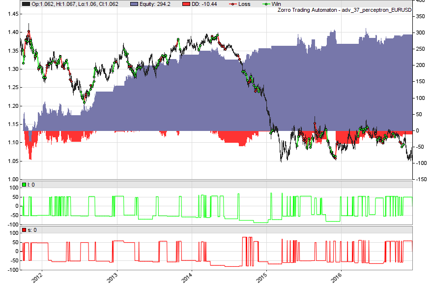 I find this result particularly interesting because I expected the perceptron to perform poorly on market data, which I find it hard to imagine falling into the linearly separable category. However, sometimes simplicity is not a bad thing, it seems.
Conclusions
I hope this article not only whet your appetite for further exploration of neural networks, but facilitated your understanding of the basic concepts, without getting too hung up on the math. I intended for this article to be an introduction to neural networks where the perceptron was to be nothing more than a learning aid. However, given the surprising walk-forward result from our simple trading model, I’m now going to experiment with this approach a little further. If this interests you too, some ideas you might consider include extending the backtest, experimenting with different signals and targets, testing the algorithm on other markets and of course considering data mining bias. I’d love to hear about your results in the comments. Thanks for reading!Free Case Study:
A wantaway engineer’s journey into professional trading and out again
I went from engineering to an equity partnership at a prop trading firm to running my own systematic trading operation from home in Western Australia.
This case study is the full story – every mistake, every breakthrough, and some things I trade today.


The line :
asset(“EUR/USD”);
might be in the wrong place.
I had to move it then the script worked.
J
Thanks Jason!
Zorro fails to compile the script if these lines are present in this shape:
var l = adviseLong(PERCEPTRON+BALANCED, ObjLong, Sig1, Sig2, Sig3, Sig4);
var s = adviseShort(PERCEPTRON+BALANCED, ObjShort, Sig1, Sig2, Sig3, Sig4);
They seem to be fine with the function syntax yet it doesn’t like it throwing series of:
Error 062: Can’t open test_nn_from_web_24.c [t:]
Commenting the adviseLong and adviseShort helps but then it doesn’t make any sense.
Error 062 occurs when Zorro can’t find a file it needs. It could be that you didn’t train your perceptrons before trying to run a backtest? During the train process, Zorro outputs the perceptron as a .c file, which is of course required before running a simulation. If that’s the case, simply hit the [Train] button on the Zorro GUI, wait for training to finish, then hit [Test].
This error can also arise when Zorro doesn’t have the correct permissions to access the files it needs. In that case, try running Zorro with Admin privileges.
” It could be that you didn’t train your perceptrons before trying to run a backtest?”
Agrh stupid me I didn’t press the button… it’s working now 😉
However it looks good only till the end of Jan 2015 – by the end the next year it lost everything.
BTW: ATR it very sensitive to the starting point of the time series: bars as old as 2000 ago can affect today results. It’s enough to shorten or lengthen the series to get different atr(10) at the end. What daily volatility almost six years ago has to today volatility? Yet it affects the atr outcome. So the dataset starting point may affect the results – did you try to move it backward or forward by a year or two?
Hello. Can we be in touch to learn more about the module