
What’s a Digital Signal?
A digital signal is a representation of physical phenomena created by sampling that phenomena at discrete time intervals. If you think about the way we typically construct a price chart, there are obvious parallels: we sample a stream of ticks at regular intervals and treat that sample as our measure of price. (Of course, we often aggregate or summarize price data at such intervals too, creating the familiar open-high-low-close bars or candles). You can, therefore, see the connection between digital signals and analysis of time-based financial data. And since the techniques used to process and make sense of digital signals have proven their worth in electrical engineering, telecommunications and other fields, it is tempting to assume that they can unravel the mysteries of the financial markets too. However, the existence of such a connection doesn’t necessarily imply that DSP holds the key to the markets, or indeed that it is of any use at all in financial applications. Financial data is much, much noisier than the data in those other applications, for example.We Need to Talk About Cycles
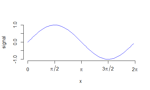
The purpose of most of the DSP tools you’ll come across, including the ones implemented in the Zorro Trading Automation Software, is to uncover useful information about some aspect of one or more cycles present in the signal being analyzed. A cycle is a repeating pattern (although non-repeating cycles can also exist), and it can be described by its:- period (\(T\)) – how much time is taken by one complete cycle.
- frequency (\(f\)) – how many times it repeats in a given time interval. Frequency and period are inversely related: \(f = \frac{1}{T}\)
- amplitude (\(A\)) – the magnitude of the distance between the peak and trough of the cycle. Often \(A\) is given as a distance from the midline to the peak (equivalently, the midline to the trough), but in Zorro’s functions it is the peak-to-trough range.
- phase (\(\theta\)) – the fraction of the cycle that has been completed at any point in time (usually measured in degrees or radians). By definition, one complete cycle occupies \(2\pi\) radians, or 360 degrees.
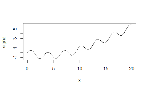
 Here’s an example of a time series with a clear cycle and trend component:
 And here’s one that I constructed by adding various trends and cycles with different amplitudes, phases and frequencies:
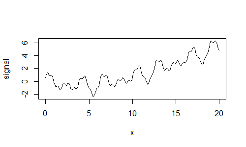 The last plot above was generated using this R code.
x <- seq(0, 20, 0.1)
signal <- 0.7*sin(2*x) - 0.001*x^3 + 0.05*x^2 - x/3 - 0.9*cos(3*x-4) + 0.3*sin(10*x)
plot(x, signal, type='l')
Note how the signal variable is constructed by simply summing multiple cycles and trends. You can see that a seemingly random looking signal can actually be decomposed into constituent cycles. In fact, using enough different cycles, you can create a good representation of any time series. The tools to do so, for example, the Fourier Transform, are well established and accessible in many software packages. But just because you can, doesn’t necessarily mean that you should. Consider that in order for our combination of cycles to be an accurate representation of a time series, they should actually be real and present in the time series. Otherwise, we are simply engaging in an exercise of overfitting, where our parameters are the constituent cycles and their properties. Since DSP is concerned with extracting information about cycles in a signal, it will be useful to the extent that there are real and present cycles in the signal.
What do you think? Are financial time series composed of multiple cycles of varying frequency and amplitude?We’ll explore this question throughout this post… There’s another potential problem in using DSP to analyze the markets, beyond the question of the fundamental existence of cycles in financial time series data. Most of the DSP techniques that you’ll encounter are particularly useful in engineering applications where the signal typically repeats – think for example of the voltage in an AC electrical circuit. Unfortunately, financial time series tend to be non-stationary and non-repeating. So, even if we accept that financial data does consist of multiple cycles that we can detect and measure, and then we do manage to detect and measure them, we are still faced with the problem of them changing through time, perhaps even before we manage to detect them!
Applications of Digital Signal Processing
Those issues aside, there may still be applications in practical trading where DSP techniques can come in handy. Consider for example some classic technical indicators like the simple moving average (SMA) and the Relative Strength Index (RSI). Both of these indicators implicitly assume some form of cyclic behaviour in the underlying time series. The SMA looks back a certain time period in its calculation, which can be interpreted as the length of the “trend” the SMA seeks to detect. (In this case, a trend is just a cycle with a long period, or equivalently a low frequency). Likewise, the RSI is calculated over a certain time period, but, in this case, its time period can be interpreted as the length of a high-frequency cycle that it seeks to detect. When viewing technical indicators from that perspective, DSP techniques may provide superior performance: they will be more responsive to the underlying data and introduce less lag than their traditional counterparts. Here’s a plot of the indicators and digital filters mentioned above (with lookback periods of 100 and 14 for the low and high-frequency indicators respectively):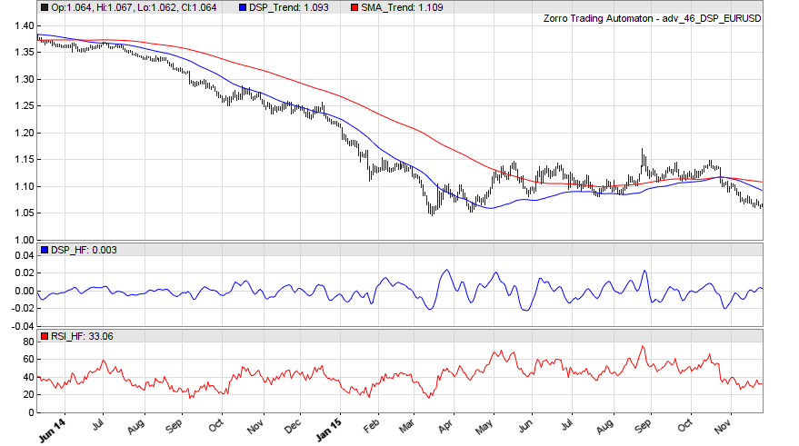 You can see that the digital filter for detecting low-frequency cycles (called a Low-Pass Filter, since it lets low-frequency cycles pass and attenuates high-frequency cycles) is more responsive and tracks price closer than the SMA.
The digital filter for detecting high-frequency cycles (called a High-Pass Filter) is smoother than the RSI and tends to emphasize turning points a little more clearly. Also notice that its output was relatively small during the period in which the market trended down, but became more pronounced as the trend ended. That’s because during the trend it correctly filtered out the low-frequency trend components of the signal which dominated during that time, hence leaving little in the output of the filter.
If nothing else, it appears that digital filters can replace certain traditional indicators. So let’s talk a little more about them.
You can see that the digital filter for detecting low-frequency cycles (called a Low-Pass Filter, since it lets low-frequency cycles pass and attenuates high-frequency cycles) is more responsive and tracks price closer than the SMA.
The digital filter for detecting high-frequency cycles (called a High-Pass Filter) is smoother than the RSI and tends to emphasize turning points a little more clearly. Also notice that its output was relatively small during the period in which the market trended down, but became more pronounced as the trend ended. That’s because during the trend it correctly filtered out the low-frequency trend components of the signal which dominated during that time, hence leaving little in the output of the filter.
If nothing else, it appears that digital filters can replace certain traditional indicators. So let’s talk a little more about them.
Exploring Digital Filters
Digital filters work by detecting cycles of various periods (lengths) in a signal, and then either attenuating (filtering) or passing those cycles, depending on their period. The cutoff period is the period at which the filter begins to attenuate the signal.- Low-Pass filters attenuate periods below their cutoff period
- High-Pass filters attenuate periods above their cutoff period.
The terminology can be a bit confusing, but just remember that Low and High refer to frequency, not period. Low frequency = long period, high frequency = short period.Another type of digital filter is the Band-Pass filter, which passes cycles with a period within a certain range (the bandwidth), and attenuates cycles outside that range. A useful way to visualize what these different filters do is to apply them to a signal with a known period and observe their output. Even better, we can supply a signal whose period gradually changes to get an even better understanding. Here’s some Zorro code for generating a sine wave with an increasing period, and plotting the output of various filters applied to this signal:
function run()
{
    set(PLOTNOW);
    MaxBars = 1000;
    asset("");
    ColorUp = ColorDn = 0;

    vars Signal = series(genSine(10, 100));
    vars LowPass50 = series(LowPass(Signal, 50));
    vars LowPass100 = series(LowPass(Signal, 100));
    vars HighPass5 = series(HighPass(Signal, 5));
    vars HighPass20 = series(HighPass(Signal, 20));
    vars BandPass40 = series(BandPass(Signal, 40, 0.1));
    vars BP4040 = series(BandPass(BandPass40, 40, 0.1));
    vars BP404040 = series(BandPass(BP4040, 40, 0.1));

    PlotHeight1 = PlotHeight2 = 150;
    PlotWidth = 800;
    plot("Signal", Signal, MAIN, BLUE);
    plot("LP50", LowPass50, NEW, RED);
    plot("LP100", LowPass100, NEW, RED);
    plot("HP5", HighPass5, NEW, RED);
    plot("HP20", HighPass20, NEW, RED);
    plot("BP40", BandPass40, NEW, RED);
    plot("BP4040", BP4040, NEW, RED);
    plot("BP404040", BP404040, NEW, RED);
}
This code outputs the following plot:
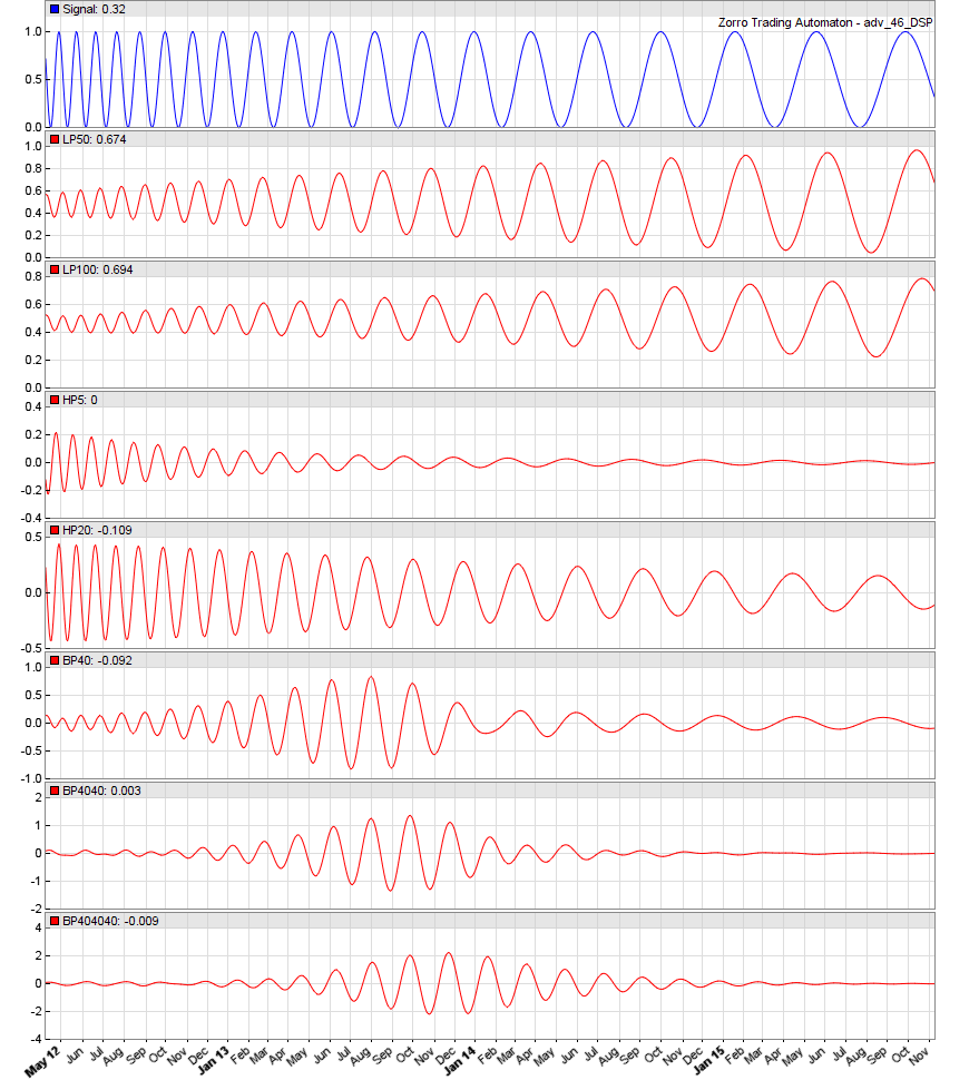 Study the plots above, and experiment with the code yourself. Note that none of the filters perfectly attenuate cycles that lie beyond their cutoff periods, although the stacked Band-Pass filters (the bottom two plots) come closer than the others do. They also introduce some lag.
In the script above, you can see that the
Study the plots above, and experiment with the code yourself. Note that none of the filters perfectly attenuate cycles that lie beyond their cutoff periods, although the stacked Band-Pass filters (the bottom two plots) come closer than the others do. They also introduce some lag.
In the script above, you can see that the BandPass function has an additional argument: as well as a cutoff period, it also takes a Delta value. The delta value is just a number between 0 and 1 that defines the width of the filter’s pass region scaled to and centred on the cutoff period.
For example, a Band-Pass filter with a cutoff period of 40 and Delta of 0.1 results in a filter with a bandwidth of 4, running from 38 to 42. It will attempt to filter cycles outside that range.
Digital filters can also be stacked by passing the output of one filter to another filter. This generally has the effect of enabling the filter to more tightly focus on the cutoff period of interest, but comes at the cost of introducing additional lag. In the script above, we demonstrated stacking a Band-Pass filter, but you can stack the other filters too. In some of the later examples, we’ll stack various filters to pre-condition our raw data before analyzing the remaining cycles. Note that doing this unavoidably introduces some amount of lag.
What CutOff Period Should I Use?
All this discussion of digital filters and their cutoff periods leads to the obvious question: what cutoff period should we use? It makes sense that if there were a dominant cycle present in the signal, that is, a cycle whose amplitude swamped the smaller cycles, we should target that cycle’s period, because it will present the best trading opportunities.The Dominant Cycle
Zorro implements theDominantPeriod function that calculates the dominant cycle period in a price series using the Hilbert Transformation.
The Hilbert Transformation is one of the fundamental functions of signal processing and enables calculation of, among other things, the instantaneous frequency of a signal.
The documentation of this function is likely to leave you scratching your head though. Testing different values of Period on a signal with a known period reveals that it has very little impact on the result and that the calculated period is quite accurate, up to a limit of around 60. My recommendation is to simply set this argument to a value of 30, which lies approximately halfway along the argument’s valid range.
Here’s a plot of the output of DominantPeriod under different conditions:
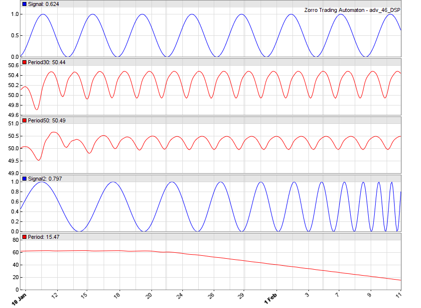
- The first signal (the top blue plot) is a sine wave of period 50.
- The next two plots are the output of DominantPeriod() with Period arguments set to 30 and 50 respectively. You can see that even when Period is set incorrectly, it does a reasonable job of extracting the cycle length.
- The second signal (blue plot, second from the bottom) is a sine wave whose period decreases from 100 to 10.
- The red plot below is the output of DominantPeriod() with Period set to 30.
 A lot of Zorro’s DSP functionality is based on the work of John Ehlers. In one of his books, Ehlers demonstrates the use of the Hilbert Transform for calculating the dominant cycle period, which is the method used in Zorro’s implementation. However, Ehlers actually warns against that approach, saying that a better method is his autocorrelation periodogram.1
Experiments with Digital Signal Processing
Let’s summarize what we’ve learned so far and then set up an experiment to look at the validity of the DSP approach in a trading context. Here’s what we know so far:- DSP tools and techniques outperform traditional indicators in terms of responsiveness and lag when used for analogous purposes.
- Digital filters can attenuate cycles of certain lengths, and pass others. We have Low-Pass filters for targeting long cycles, High-Pass filters for targeting short cycles, and Band-Pass filters for targeting a range of cycle lengths. Filters can be connected, or stacked. This often improves their accuracy but comes at the expense of added lag.
- We can estimate the period of the dominant cycle using Zorro’s DominantPeriod() function, which lags by approximately ten bars.
- At the heart of the indicator is a Band-Pass filter of an arbitrary bandwidth.
- Preceding the Band-Pass filter, the raw price series is passed to a High-Pass filter that is tuned to twice the period of the Band-Pass filter’s upper cutoff. That’s to remove the effects of spectral dilation, which Ehlers says arises due to the phenomenon that market swings tend to be larger in amplitude the longer they are measured over.
- Finally, the output of the Band-Pass filter is fed to another High-Pass filter, this time tuned to the other side of the Band-Pass filter’s bandwidth. The output of this High-Pass filter, according to Ehlers, creates a waveform that leads the Band-Pass filter’s output and will cross that output at its exact peaks and valleys, except when the data are trending.3We’ll refer to this leading waveform as our trigger.
/* DSP Experiments from Cycle Analytics For Traders

Note Ehlers often speaks in frequency terms, we work in period terms
High frequency = low cutoff period
Low frequency = high cutoff period

*/

function run()
{
    set(PLOTNOW);
    StartDate = 2007;
    EndDate = 2016;
    BarPeriod = 60;
    LookBack = 250;
    MaxLong = MaxShort = 1;

    while(asset(loop("EUR/USD", "USD/JPY", "SPX500")))
    while(algo(loop("H1", "H4", "D1")))
    {
        if(Algo == "H1") TimeFrame = 60/BarPeriod;
        else if(Algo == "H4") TimeFrame = 240/BarPeriod;
        else if(Algo == "D1") TimeFrame = 1440/BarPeriod;

        Spread = Commission = Slippage = RollLong = RollShort = 0;

        vars Price = series(price());

        // Set up filter parameters
        int BP_Cutoff = 30;
        var Delta = 0.3;
        int Bandwidth = ceil(BP_Cutoff*Delta);
        int UpperBP_Cutoff = ceil(BP_Cutoff + Bandwidth/2);
        int LowerBP_Cutoff = floor(BP_Cutoff - Bandwidth/2);

        if(Day == StartBar and Asset == "EUR/USD" and Algo == "H1")
            printf("\nFilter Bandwith is %d to %d Periods", LowerBP_Cutoff, UpperBP_Cutoff);

        // Pre-filter with High-Pass filter
        vars HP = series(HighPass(Price, UpperBP_Cutoff*2));

        // Band-Pass filter
        vars BP = series(BandPass(HP, BP_Cutoff, Delta));

        // Trigger: another High-Pass filter
        vars Trigger = series(HighPass(BP, LowerBP_Cutoff));

        // Trade logic
        if(crossOver(Trigger, BP)) enterLong();
        if(crossUnder(Trigger, BP)) enterShort();

        plot("BP", BP, NEW, BLUE);
        plot("Trigger", Trigger, 0, RED);

    }
}

/* OUTPUT:
Portfolio analysis  OptF  ProF  Win/Loss  Wgt%

EUR/USD avg         .003  0.94  2018/1611   18.9
SPX500 avg          .003  0.88  1824/1522   58.0
USD/JPY avg         .000  0.88  1946/1637   23.1

D1 avg              .002  0.90  184/157   12.1
H1 avg              .000  0.88  4449/3693   71.9
H4 avg              .005  0.95  1155/920   16.0

EUR/USD:D1          .000  0.79   61/52     9.6
EUR/USD:D1:L        .000  0.68   32/24     7.8
EUR/USD:D1:S        .000  0.91   29/28     1.8
EUR/USD:H1          .000  0.96  1538/1244    8.1
EUR/USD:H1:L        .000  0.93  786/605    7.0
EUR/USD:H1:S        .000  0.99  752/639    1.1
EUR/USD:H4          .000  0.99  419/315    1.2
EUR/USD:H4:L        .000  0.93  210/157    3.5
EUR/USD:H4:S        .027  1.05  209/158   -2.4
SPX500:D1           .000  0.98   54/51     0.8
SPX500:D1:L         .016  1.40   32/21    -8.5
SPX500:D1:S         .000  0.70   22/30     9.3
SPX500:H1           .000  0.84  1427/1173   47.3
SPX500:H1:L         .000  0.89  766/534   15.1
SPX500:H1:S         .000  0.80  661/639   32.2
SPX500:H4           .000  0.93  343/298    9.9
SPX500:H4:L         .004  1.05  195/126   -3.6
SPX500:H4:S         .000  0.82  148/172   13.5
USD/JPY:D1          .000  0.93   69/54     1.7
USD/JPY:D1:L        .000  0.89   32/30     1.2
USD/JPY:D1:S        .000  0.96   37/24     0.5
USD/JPY:H1          .000  0.86  1484/1276   16.5
USD/JPY:H1:L        .000  0.85  744/636    8.6
USD/JPY:H1:S        .000  0.86  740/640    8.0
USD/JPY:H4          .000  0.92  393/307    4.9
USD/JPY:H4:L        .000  0.91  196/154    2.8
USD/JPY:H4:S        .000  0.93  197/153    2.1
*/
Not much to like about that at all. Just for completeness, here’s the equity curve:
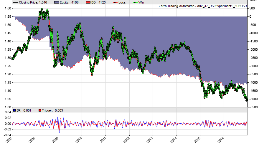 This result feels like we are almost completely out of sync with the cycles we are trying to exploit! Either that or the cycles are just randomness and can’t be exploited anyway. Let’s explore some more.
In this case, the bandwidth of our Band-Pass filter was tuned to periods of length 25 to 35. That’s neither a very wide range, nor are those particularly long cycles.
Perhaps if we increase both our Band-Pass cutoff period and the Delta parameter in order to target longer cycles we can get better results?
Here’s the portfolio report for a Band-Pass cutoff of 50 and a Delta of 0.8, which corresponds to a bandwidth that encompasses cycles of length 30 to 70 bars:
This result feels like we are almost completely out of sync with the cycles we are trying to exploit! Either that or the cycles are just randomness and can’t be exploited anyway. Let’s explore some more.
In this case, the bandwidth of our Band-Pass filter was tuned to periods of length 25 to 35. That’s neither a very wide range, nor are those particularly long cycles.
Perhaps if we increase both our Band-Pass cutoff period and the Delta parameter in order to target longer cycles we can get better results?
Here’s the portfolio report for a Band-Pass cutoff of 50 and a Delta of 0.8, which corresponds to a bandwidth that encompasses cycles of length 30 to 70 bars:
Portfolio analysis  OptF  ProF  Win/Loss  Wgt%

EUR/USD avg         .019  1.01  1156/817    4.2
SPX500 avg          .012  1.21  1145/771   79.9
USD/JPY avg         .024  1.10  1214/798   15.9

D1 avg              .024  1.34  117/75    32.2
H1 avg              .018  1.06  2683/1848   28.5
H4 avg              .019  1.16  715/463   39.3

EUR/USD:D1          .008  1.04   35/29     1.5
EUR/USD:D1:L        .000  0.86   18/14    -3.1
EUR/USD:D1:S        .074  1.36   17/15     4.6
EUR/USD:H1          .000  0.98  891/628   -2.7
EUR/USD:H1:L        .000  0.95  452/307   -4.9
EUR/USD:H1:S        .023  1.03  439/321    2.2
EUR/USD:H4          .026  1.06  230/160    5.5
EUR/USD:H4:L        .000  0.98  119/76    -0.8
EUR/USD:H4:S        .055  1.15  111/84     6.3
SPX500:D1           .012  1.59   33/25    23.2
SPX500:D1:L         .015  2.66   21/8     22.4
SPX500:D1:S         .001  1.03   12/17     0.7
SPX500:H1           .015  1.11  869/604   25.4
SPX500:H1:L         .023  1.21  468/268   22.9
SPX500:H1:S         .003  1.02  401/336    2.4
SPX500:H4           .020  1.28  243/142   31.4
SPX500:H4:L         .027  1.51  131/62    25.9
SPX500:H4:S         .007  1.09  112/80     5.4
USD/JPY:D1          .028  1.36   49/21     7.6
USD/JPY:D1:L        .029  1.38   26/9      3.6
USD/JPY:D1:S        .027  1.35   23/12     4.0
USD/JPY:H1          .031  1.06  923/616    5.9
USD/JPY:H1:L        .027  1.06  464/305    2.5
USD/JPY:H1:S        .034  1.07  459/311    3.3
USD/JPY:H4          .014  1.05  242/161    2.4
USD/JPY:H4:L        .009  1.03  117/85     0.7
USD/JPY:H4:S        .018  1.07  125/76     1.7
Interesting. This appears to be a better result, although long trades on SPX500 contributed the majority of the profit. Still, maybe this deserves a closer look. Here’s the portfolio equity curve:

Incorporating the Period of the Dominant Cycle
Ehlers says later in his book4that it makes sense to tune the Band-Pass filter to the dominant cycle in order to eliminate other cycles that are of little or no interest. He then goes on to say that even better than tuning it to dominant cycle, tuning it to a slightly shorter period (but with a bandwidth that also captures the dominant cycle) causes the output of the filter to lead the dominant cycle slightly. We test this idea in the code below (the tuning of the Band-Pass filter as described above occurs in line 34). In this case, Ehlers suggests that we precede the Band-Pass filter with what he calls a Roofing Filter, which is simply a High-Pass and Low-Pass filter connected in series for pre-conditioning the data and removing unwanted cycles. Zorro implements the Roofing Filter as the function Roof() and we use it here. Our trigger line is calculated as 90% of the amplitude of the 1-bar lagged Band-Pass filter output. The “strategy” now does the following:- Pre-processes the raw price series using Ehlers’ Roofing Filter
- Calculates the period of the dominant cycle of the pre-processed price series
- Tunes a Band-Pass filter centred on a period slightly lower than the dominant cycle, but with a bandwidth that incorporates the dominant cycle.
- Calculates a trigger line based on 90% of the one-bar lagged Band-Pass filter output.
- We simply reverse long and short when the trigger line crosses under and over the Band-Pass output respectively.
/* DSP Experiments from Cycle Analytics For Traders

Note Ehlers often speaks in frequency terms, we work in period terms
High frequency = low cutoff period
Low frequency = high cutoff period

*/

function run()
{
    set(PLOTNOW);
    StartDate = 2007;
    EndDate = 2016;
    BarPeriod = 60;
    LookBack = 200*24;
   MaxLong = MaxShort = 1;

    while(asset(loop("EUR/USD", "USD/JPY", "SPX500")))
    while(algo(loop("H1", "H4", "D1")))
    {
        if(Algo == "H1") TimeFrame = 60/BarPeriod;
        else if(Algo == "H4") TimeFrame = 240/BarPeriod;
        else if(Algo == "D1") TimeFrame = 1440/BarPeriod;

        Spread = Commission = Slippage = RollLong = RollShort = 0;

        vars Price = series(price());

        // Pre-filter with High-Pass filter
        vars HP = series(Roof(Price, 10, 70));

        // Set up filter parameters
        var DomPeriod = DominantPeriod(HP, 30);
        var Delta = 0.3;
        var BP_Cutoff = (1 - 2/3*(0.5 * Delta)) * DomPeriod; //tune to a shorter period
        int Bandwidth = ceil(BP_Cutoff*Delta);
        int UpperBP_Cutoff = ceil(BP_Cutoff + Bandwidth/2);
        int LowerBP_Cutoff = floor(BP_Cutoff - Bandwidth/2);

        // Band-Pass filter
        vars BP = series(BandPass(HP, BP_Cutoff, Delta));

        // Trigger: another High-Pass filter
        vars Trigger = series(0.9*BP[1]);

        // Trade logic
        if(crossOver(Trigger, BP)) enterLong();
        if(crossUnder(Trigger, BP)) enterShort();

        plot("BP", BP, NEW, BLUE);
        plot("Trigger", Trigger, 0, RED);
        plot("DomCyclePeriod", DomPeriod, NEW, BLACK);
        plot("UpperCutoff", UpperBP_Cutoff, 0, RED);
        plot("LowerCutoff", LowerBP_Cutoff, 0, RED);
    }
}

/* OUTPUT
Portfolio analysis  OptF  ProF  Win/Loss  Wgt%

EUR/USD avg         .031  1.04  3325/2678   22.0
SPX500 avg          .014  1.11  3079/2753   80.0
USD/JPY avg         .006  0.99  3262/2758   -2.0

D1 avg              .021  1.23  325/268   39.2
H1 avg              .020  1.04  7420/6351   36.2
H4 avg              .020  1.05  1921/1570   24.6

EUR/USD:D1          .049  1.18  113/91    11.2
EUR/USD:D1:L        .000  1.00   53/49    -0.1
EUR/USD:D1:S        .090  1.40   60/42    11.3
EUR/USD:H1          .041  1.03  2559/2057    8.8
EUR/USD:H1:L        .000  0.99  1282/1026   -1.1
EUR/USD:H1:S        .092  1.07  1277/1031    9.9
EUR/USD:H4          .009  1.01  653/530    2.0
EUR/USD:H4:L        .000  0.95  330/261   -4.5
EUR/USD:H4:S        .068  1.09  323/269    6.5
SPX500:D1           .023  1.44  114/78    31.4
SPX500:D1:L         .027  1.78   68/28    25.5
SPX500:D1:S         .010  1.15   46/50     5.9
SPX500:H1           .015  1.07  2349/2160   29.5
SPX500:H1:L         .022  1.11  1246/1009   23.9
SPX500:H1:S         .006  1.02  1103/1151    5.5
SPX500:H4           .011  1.09  616/515   19.2
SPX500:H4:L         .018  1.17  336/229   18.8
SPX500:H4:S         .000  1.00  280/286    0.4
USD/JPY:D1          .000  0.91   98/99    -3.4
USD/JPY:D1:L        .000  0.91   48/51    -1.7
USD/JPY:D1:S        .000  0.92   50/48    -1.7
USD/JPY:H1          .000  0.99  2512/2134   -2.1
USD/JPY:H1:L        .000  0.99  1266/1057   -1.0
USD/JPY:H1:S        .000  0.99  1246/1077   -1.1
USD/JPY:H4          .018  1.04  652/525    3.5
USD/JPY:H4:L        .020  1.04  321/267    1.8
USD/JPY:H4:S        .016  1.04  331/258    1.6
*/
And here’s the equity curve (I also plotted the upper and lower range of the Band-Pass filter’s bandwidth around the dominant cycle):
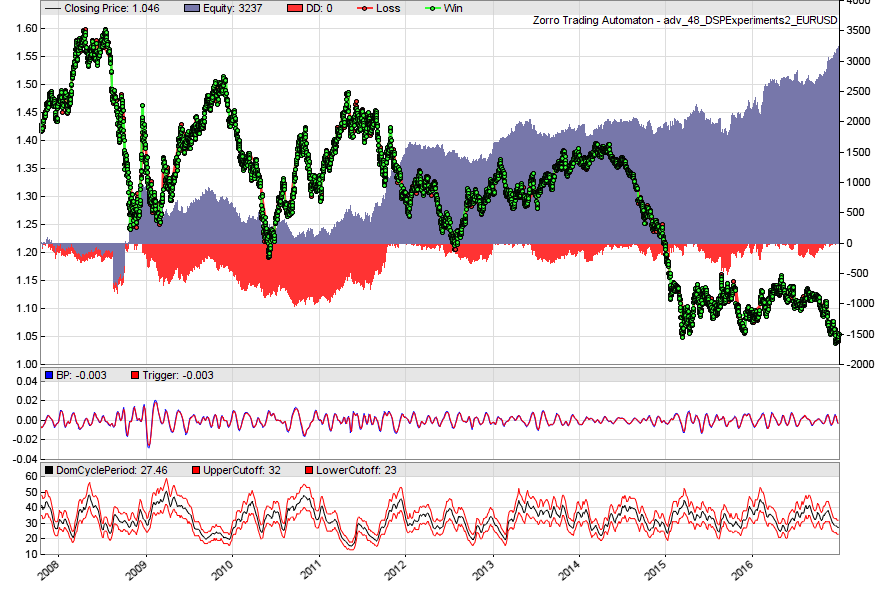 It occurred to me that maybe we want to avoid reversing our trades when the dominant cycle turns into a trend. When that happens, wouldn’t we want to hold onto our current trade, rather than reversing?
Now, recall that our DominantPeriod() function topped out at a cycle period of around 60 bars. It couldn’t detect any cycles longer than that period effectively (go back and look at the plots of the sine waves and the output of DominantPeriod() above if you’re unsure).
That means that at the upper end of DominantPeriod() ‘s output range, we have a significant amount of uncertainty about the actual dominant cycle period: it could be 60 bars, it could be 160 bars, DominantPeriod() would output roughly the same value in either case.
To test this, we can simply prevent the reversing of our positions when DominantPeriod() approaches the upper boundary of its range. That will mean that any currently open trade will stay open until DominantPeriod() detects a shorter cycle, hopefully exploiting any cycles that turn into trends. Just replace the trade logic (lines 45-47) with this code:
It occurred to me that maybe we want to avoid reversing our trades when the dominant cycle turns into a trend. When that happens, wouldn’t we want to hold onto our current trade, rather than reversing?
Now, recall that our DominantPeriod() function topped out at a cycle period of around 60 bars. It couldn’t detect any cycles longer than that period effectively (go back and look at the plots of the sine waves and the output of DominantPeriod() above if you’re unsure).
That means that at the upper end of DominantPeriod() ‘s output range, we have a significant amount of uncertainty about the actual dominant cycle period: it could be 60 bars, it could be 160 bars, DominantPeriod() would output roughly the same value in either case.
To test this, we can simply prevent the reversing of our positions when DominantPeriod() approaches the upper boundary of its range. That will mean that any currently open trade will stay open until DominantPeriod() detects a shorter cycle, hopefully exploiting any cycles that turn into trends. Just replace the trade logic (lines 45-47) with this code:
// Trade logic
if(DomPeriod < 45)
{
    if(crossOver(Trigger, BP)) enterLong();
    if(crossUnder(Trigger, BP)) enterShort();
}
Here’s the resulting equity curve; the boost in performance is obvious and not insignificant:

Spectral Analysis and the Fourier Transform
The Fourier Transform is another fundamental operation of DSP. It is used to:- Decompose a signal into its component cycles, and
- Determine the contribution of each cycle to the signal
Plotting the Spectrum of Frequencies
A plot of the contribution of each cycle to a signal is referred to as the signal’s frequency spectrum. Zorro has a tool for creating such plots. I mentioned above that one of the confounding factors in the application of DSP to financial time series is that such series are typically non-stationary. That means that the frequency spectrum calculated over one period may be completely different over another.How different?Well, we already saw in our use of the DominantPeriod() function that the strongest cycle tended to wander around quite a bit. Let’s find out what analysis of the frequency spectrum says about that. To plot the frequency spectrum of a price series, we need to use the Spectrum() function. This function calculates the relative contribution of a single cycle to the overall signal. If we plot the contribution of several different cycles, we’ll see just how unstable the relative contributions are. Here’s some code for plotting the contribution of the 24, 48, 72, 96 and 120 hour cycles to the EUR/USD over a few years:
/* SPECTRAL ANALYSIS

*/

function run()
{
    set(PLOTNOW);
    StartDate = 20120101;
    EndDate = 2016;
    LookBack = 120*5;

    vars Price = series(price());

    PlotHeight1 = 200;
    PlotHeight2 = 100;
    int i;
    for(i=24; i<121; i+=24)
    {
        plot(strf("Spectrum_%d", i), Spectrum(Price, i, i*5), NEW, color(100*i/120, BLUE, DARKGREEN, RED, BLACK));
    }

}
And here’s the plot:
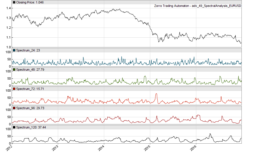 You can see that the relative contributions (or amplitude, or strength) of these cycles are anything but constant.
I wanted to show you this plot as a first step in exploring frequency spectra because often you’ll see a histogram or some other plot that shows the relative contributions of all the cycles over some period of time.
If you haven’t seen a plot like the one above, you could be forgiven for assuming that such a histogram describes general characteristics of a market: in fact, what it really shows is just a snapshot in time.
Let’s build one such snapshot in time. To do that, we call Spectrum() for every cycle period that we are interested in (inside a for() loop) and plot its relative contribution as a bar in a histogram. Here’s the code to do just that, where we plot the spectrum for a single 3-month period:
You can see that the relative contributions (or amplitude, or strength) of these cycles are anything but constant.
I wanted to show you this plot as a first step in exploring frequency spectra because often you’ll see a histogram or some other plot that shows the relative contributions of all the cycles over some period of time.
If you haven’t seen a plot like the one above, you could be forgiven for assuming that such a histogram describes general characteristics of a market: in fact, what it really shows is just a snapshot in time.
Let’s build one such snapshot in time. To do that, we call Spectrum() for every cycle period that we are interested in (inside a for() loop) and plot its relative contribution as a bar in a histogram. Here’s the code to do just that, where we plot the spectrum for a single 3-month period:
* SPECTRAL ANALYSIS

*/

function run()
{
    set(PLOTNOW);
    StartDate = 20160101;
    EndDate = StartDate + 00000300;
    LookBack = 120*2;

    vars Price = series(price());
    vars Rand = series(0);
    if(is(LOOKBACK))
        Rand[0] = Price[0];
    else
        Rand[0] = Rand[1] + random(0.005)*random();

//  plot("random", Rand, MAIN, BLUE);

    PlotWidth = 800;
    PlotHeight1 = 350;
    int Period;
    for(Period = 6; Period < 120; Period += 1)
    {
        plotBar("Spectrum",Period,Period,Spectrum(Price,Period,2*Period),BARS+AVG+LBL2,DARKGREEN);
    }
}
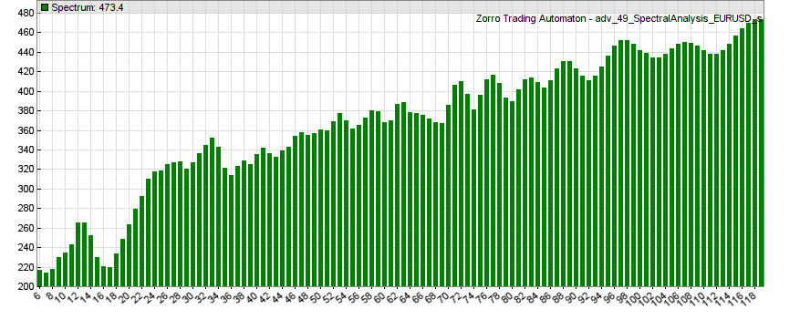
Here’s the plot for EUR/USD:
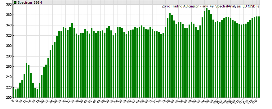
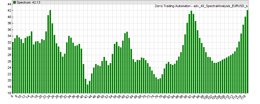 If we advance the script to look at the next three-month period, we get this plot:
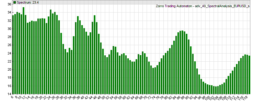 There are definite peaks in the frequency spectra plots, which suggests that certain cycles do in fact exist in this market.
However, you can see that for the most part, they are not constant, and some peaks shift more than others.
If you repeat the analysis over different periods (months, weeks, or years) you’ll find other shifting, ephemeral, but clearly visible cycles.
There are definite peaks in the frequency spectra plots, which suggests that certain cycles do in fact exist in this market.
However, you can see that for the most part, they are not constant, and some peaks shift more than others.
If you repeat the analysis over different periods (months, weeks, or years) you’ll find other shifting, ephemeral, but clearly visible cycles.
Aren’t we just seeing random patterns here?
But couldn’t those peaks just be random fluctuations? What evidence is there that they are real cycles, and not just an artefact of randomness? Well, we can construct a random price curve that starts at the same level as our real price curve and changes with roughly the same volatility, but does so using a random number generator. Then, we can plot the frequency spectrum of that random price curve and see if we get similar fluctuations. I already added the code to create the random price series (lines 13-17 in the script above). To test it, just replace Price with Rand in the Spectrum() function. Here’s a plot of one realization of that random price curve (blue), overlaid with the real one (black):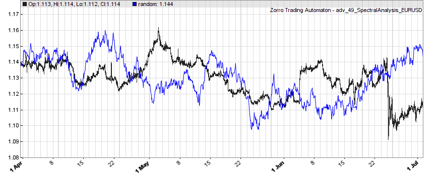 Looks pretty believable, doesn’t it? Visual inspection certainly suggests that it could pass for a real price series. Let’s see what sort of frequency spectrum such a random price curve generates:
 Not really the same as the one generated by our real price curve.
Here’s another one in case the first one was a fluke (every time you run the code above, you’ll get a different random price curve, and I encourage you to test this yourself):
Not really the same as the one generated by our real price curve.
Here’s another one in case the first one was a fluke (every time you run the code above, you’ll get a different random price curve, and I encourage you to test this yourself):
 This hints that the cycles evident in the frequency spectrum of our price curve are not just random artefacts.
If we were convinced by this, then the challenge we would face is overcoming their shifting and ephemeral nature in order to take advantage of these cycles.
This hints that the cycles evident in the frequency spectrum of our price curve are not just random artefacts.
If we were convinced by this, then the challenge we would face is overcoming their shifting and ephemeral nature in order to take advantage of these cycles.
Is Digital Signal Processing Useful to the Quant Trader?
I take a somewhat measured attitude to using DSP as an approach to the markets. We have seen that some financial time series appear to exhibit cyclical behaviour and are therefore candidates for exploitation using tools and techniques that can identify and quantify those cycles. The challenge we face is that those cycles – if they even exist – are not constant in time. Our analysis suggests that – even if they are not just random – these cycles are constantly shifting, evolving, appearing and disappearing, and will show up in different ways depending on the lens through which you view the markets. That’s no small challenge to overcome. While it is possible that cycle decomposition, done skillfully, may yield good results, DSP is certainly more readily useful for replacing or upgrading traditional technical indicators. This in spite of the fact that non-stationary, and non-repeating financial data is something of a departure from the typical use cases of these techniques – perhaps because traditional indicators are already burdened with that particular shortcoming, in addition to their sub-optimal lag and attenuation characteristics. If you wanted to take this approach further, you might want to look at the concept of wavelet decomposition. Wavelets are used to decompose a signal, much like the Fourier Transform, but do so in both the frequency and time domains. They may, therefore, be more useful than the frequency (equivalently, period) based decomposition we looked at here. In addition, there are other time-frequency decompositions which could be explored as well. If you are interested in pursuing wavelets for applications in algorithmic trading, expect to do a lot of research, particularly if you are new to DSP. That’s not meant to scare you off, rather I just want to give you a taste of what’s out there and set some realistic expectations.
Finally, there’s one other method that belongs partially to DSP, but probably more to control theory: the Kalman filter, which finds application in trading strategies like this one.
Free Case Study:
A wantaway engineer’s journey into professional trading and out again
I went from engineering to an equity partnership at a prop trading firm to running my own systematic trading operation from home in Western Australia.
This case study is the full story – every mistake, every breakthrough, and some things I trade today.


It is very interesting, great article on the topic of DSP that I understand far better now.
Thank you so much for writing this! I saw a Pine Script tutorial on DSP a few months ago but it didn’t mention at all how any of it could be applied to trading! Then randomly I was drawing trend lines through the candles, and the way price oscillated around certain prices reminded me of audio wave forms, I googled signal processing and trading and this article came up…I recorded and engineered music for years…NEVER thought in a trillion years you could use a low pass filter to find trading signals. What can’t you use a filter for??? I think that’s the more relevant question now….Will it help me get a better tax deduction? Will a high pass help me lose weight? This article is mind blowing. I wish more people could see this. You and Ehler are amazing people for sharing this knowledge.