The Law of Large Numbers – Part 2

This is Part 2 in our Practical Statistics for Algo Traders blog series—don’t forget to check out Part 1 if you haven’t already.

Even if you’ve never heard of it, the Law of Large Numbers is something that you understand intuitively, and probably employ in one form or another on an almost daily basis. But human nature is such that we sometimes apply it poorly, often to great detriment. Interestingly, psychologists found strong evidence that, despite the intuitiveness and simplicity of the law, humans make systematic errors in its application. It turns out that we all tend to make the same mistakes – even trained statisticians who not only should know better, but do!

In 1971, two Israeli psychologists, Amos Tversky and Daniel Kahneman,1Readers of the Robot Wealth blog will know that I’m a big fan of the work of Tversky and Kahneman. In fact, I’d go as far to call it the most important body of work related to understanding errors made by the human mind – something that is of obvious interest to traders. Check out Kahneman’s “Thinking Fast and Slow” for a dense but readable summary of their work, or Michael Lewis’ “The Undoing Project” for more of a narrative style approach. published “Belief in the law of small numbers“, reporting that

People have erroneous intuitions about the laws of chance. In particular, they regard a sample randomly drawn from a population as highly representative, that is, similar to the population in all essential characteristics.

So what is this Law of Large Numbers? What are the consequences of a misplaced belief in the law of small numbers? And what does it all mean for algo traders? Well, to answer these questions, we first need to talk about burgers.

The Law of Large Numbers Explained

Put simply, the Law of Large Numbers states that if we select a sample from an entire population, the mean of our sample approaches the mean of the population as we increase our sample size. Said differently, the greater our sample size, the less uncertainty we have regarding our conclusions  about the population.

We all understand this law on an intuitive level. For instance, say you’re looking at reviews of burger joints in your local area. You come across a place that only has two reviews, both of them rating the restaurant 5 out of 5. There’s another place that has an average rating of 4.7, but it has 200 reviews.

You know instinctively that the place rated 4.7 is the most likely of the two to dish up a fantastic burger, even though it’s average rating is less than the perfect 5 of the first restaurant. That’s the law of large numbers in action.

How many reviews would it take before you started considering that there was a good chance that the first burger joint served better burgers than the second? 5? 10? 100?

Let’s assume that the burger joint with the perfect record after two reviews is actually destined for a long-term average rating of just over 4. We could simulate several thousand reviews whose aggregate characteristics match this assumption with the following R code:

library(ggplot2)

# burger joint destined for a long-term average rating of around 4 out of 5
probs <- c(0.025, 0.05, 0.125, 0.5, 0.35)
probs <- probs/(sum(probs))
ratings <- c(1, 2, 3, 4, 5)
p <- sum(probs*ratings)

reviews <- sample(1:5, 5000, replace=TRUE, prob=probs)
mean(reviews)

ggplot() + aes(reviews) + 
  geom_histogram(binwidth=1,
                 col="black", 
                 fill="blue", 
                 alpha = .75) + 
  labs(title="Histogram of Ratings", x="Rating", y="Count")

And here’s a histogram of the simulated reviews – note that the rating most often received was 4 out of 5:

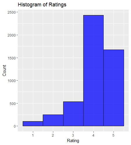The output of the simulation gives us a “population” of reviews for our burger joint. Next we’re interested in the uncertainty associated with a small number of reviews – a “sample” drawn from the “population”. How representative are our samples of the population? In particular, how many reviews do we need in order to reflect the actual mean of 4?

To answer that, we can  turn again to simulation. The following R code samples the synthetic reviews we created above repeatedly for various sample sizes, and then plots the results in a scatter plot. You can see the true average rating as a black line, and the the other restaurant’s 200-review average as a dashed red line:

# average rating given num_reviews ratings
num_reviews <- sample(c(1:100), 10000, replace=TRUE)
average_rating <- c()
for(i in c(1:length(num_reviews))) {
  average_rating[i] <- mean(sample(reviews, num_reviews[i], replace=FALSE))
}

# plot
ggplot() + aes(x=num_reviews, y=average_rating) +
  geom_point(color="blue", alpha=0.5) +
  geom_hline(yintercept=p, color="black", size=1, show.legend = TRUE) +
  geom_hline(yintercept=4.7, color="red", linetype="dashed", size=1) +
  labs(title="Convergence of Sample Mean to Population Mean", x="Number of Reviews", y="Average Rating") +
  annotate("text", x=80, y=p-0.1, label="True average rating", size=8) + 
  annotate("text", x=85, y=4.9, label="Other restaurant's average rating", size=8)

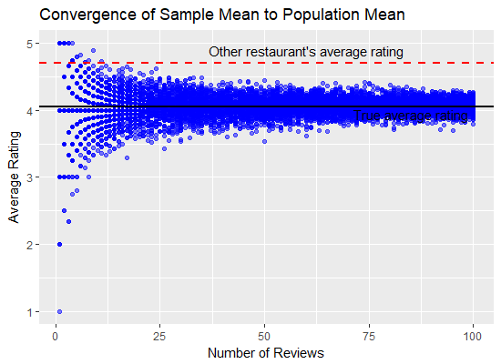We can see that as the sample size grows, the spread in the average rating decreases, and starts to converge around the true average rating. At a sample size of 100 reviews, we could conceivably end up with an average rating of anywhere between about 3.75 and 4.25.

But look at what happens when our sample size is small! Even with 50 reviews, it’s possible that the sample’s average grossly over- or under-estimates the true average.

We can see that with a sample of 10 reviews, it’s possible that we end up with a sample average that exceeds the average of the gourmet, 4.7-star restaurant. But even out to about 25 reviews, we could still end up with an average rating that isn’t all that distinguishable either.

Even when we have 100 reviews, there exists a level of uncertainty around the sample average. But the uncertainty with 100 reviews is much less than with 10 reviews. But the point is it still exists! We run into problems because, according to Kahneman and Tversky, we tend to grossly misjudge this uncertainty, in many cases ignoring it altogether!

Personally, I try to incorporate uncertainty into my thinking about most things in life, not just burgers and trading. But Kahneman and Tversky make the point that even when we do this, we tend to muck it up! A more robust solution is to use a quantitative approach to factoring uncertainty into decision making. Bayesian reasoning is a wonderful paradigm for doing precisely this, but that’s a topic for another time. Here, I merely want to share with you some examples and applications related to trading.

So to conclude our treatise on burger reviews, if we are comparing burger joints under a 5-star review system, eyeballing the scatterplot above suggests we need about 25 reviews for a new restaurant whose (at the time unknown) long-term average is 4 stars before we can be fairly sure  that it’s burgers won’t be quite as tasty as our tried and tested 4.7-star Big Kahuna burger joint.

Why the Law of Large Numbers Matters to Traders

As much as I’m sure you enjoy thinking about the statistics of burger review systems, let’s turn our attention to trading. In particular, I want to show you how our intuition around the law of large numbers can lead us to make bad decisions in our trading, and what to do about it.

High-frequency trading strategies typically have a much higher Sharpe ratio than low frequency strategies, since the variability of returns is generally much higher in the latter. If you had a high-frequency strategy with a Sharpe ratio in the high single digits, you’d only need to see a week or two of negative returns – perhaps less – to be quite sure that your strategy was broken.

But most of us don’t have the capital or infrastructure to realise a high-frequency strategy. Instead, we trade lower frequency strategies and accept that our Sharpe ratios are going to be lower as well. In my experience, a typical non-professional might consider trading a strategy with a Sharpe between about 1.0 and 2.0.

How long does it take to realise such a strategy’s true Sharpe? And how much could that Sharpe vary when measured on samples of various sizes? The answer, which we’ll get too shortly, might surprise you, or even scare you! Because it turns out that a “large” number may or may  not be so large, depending on the context. And that lack of context awareness is precisely where we tend to make our  most severe errors in the application of the Law of Large Numbers.

First of all, let’s simulate various realisations of 40 days of trading a strategy with a true Sharpe ratio of 1.5. This is equivalent to around two months of trading.

If we set the strategy’s mean daily return, mu , to 0.1%, we can calculate the standard deviation of returns, sigma , that results in a true Sharpe of 1.5:

# backtested strategy has a sharpe of 1.5
# sqrt(252)*mu/sigma = 1.5

mu <- 0.1/100
sigma <- mu*sqrt(252)/1.5

And here’s 5,000 realisations of 40 days of trading a strategy with this performance (under the assumption that daily returns are normally distributed, an inaccurate but convenient simplification that won’t detract too much from the point):

N <- 5000
days <- 40
sharpes <- c()
for(i in c(1:N)) {
  daily_returns <- rnorm(days, mu, sigma)
  # sharpe of simulated returns
  sharpes[i] <- sqrt(252)*mean(daily_returns)/sd(daily_returns)
}

Whoa! The histogram shows that it isn’t inconceivable (in fact it’s quite likely) that our Sharpe 1.5 strategy could give us an annualised Sharpe of -2 or less over a 40-day period!

What would you do if the strategy you’d backtested to a Sharpe of 1.5 had delivered an annualised Sharpe of -2 over the first two months of trading? Would you turn it off? Tinker with it? Maybe adjust a parameter or two?

You should probably do nothing! At least until you’ve assessed the probability of your strategy delivering the actual results, assuming it’s performance was indeed what you’d backtested it to be. To do that, you can just sum up the number of simulated 40-day Sharpes that were less than or equal to -2, and then divide by the number of Sharpes we simulated:

# probability of getting sharpe of -2 or less in 40 days
100*sum(sharpes <= -2)/N

which works out to about 8.5%.

Let’s now look at the convergence of our Sharpe ratio to the expected Sharpe as we increase the sample size, just as we did in the burger review example above. Here’s the code:

trading_days <- sample(10:500, 5000, replace=TRUE) # sample of 10-1000 trading days
sharpes <- c()
for(i in c(1:length(trading_days))) {
  daily_returns <- rnorm(trading_days[i], mu, sigma)
  sharpes[i] <- sqrt(252)*mean(daily_returns)/sd(daily_returns)
}

ggplot() + aes(x=trading_days, y=sharpes) +
  geom_point(color="blue", alpha=0.5) +
  geom_hline(yintercept=1.5, color="red", linetype="dashed", size=1) +
  labs(title="Convergence of Sample Mean to Population Mean", x="Number of Trading Days", y="Sharpe") +
  annotate("text", x=85, y=p-0.1, label="True Sharpe", size=4)

And the output:

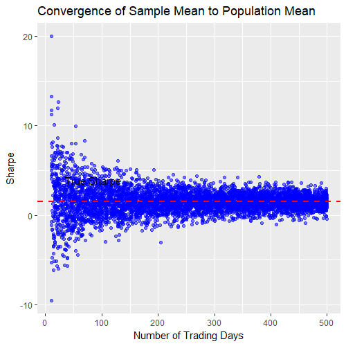Once again we see the sample uncertainty shrink as we increase the sample size, but this time it’s magnitude looks much more frightening. Note the uncertainty even after 500 trading days! This implies that our strategy with a long-term Sharpe of 1.5 could conceivably deliver very small or even negative returns in a two-year period.

If you’ve done a lot of backtesting, you probably understand from experience that a strategy with a Sharpe of 1.5 can indeed have drawdowns that last one or two years. So maybe this result doesn’t surprise you that much. But consider how you’d feel and act in real time if you suffered through such a drawdown after going live with this strategy that you’d painstakingly developed. Would you factor the uncertainty of the sample size into your decision making?

The point is that this time the uncertainty really matters. Maybe you don’t care that much if you thought you were getting a 5-star burger, but ended up eating a 4-star offering. You could probably live with that. But what if you were expecting to realise your Sharpe 1.5 strategy, but after 2 years you’d barely broken even?

Returning to our 40-days of unprofitable trading of our allegedly profitable strategy. As mentioned above, there’s an 8.5% chance of getting an annualised Sharpe of -2 from this scenario. Maybe that’s enough to convince you that your strategy is not actually going to deliver a Sharpe of 1.5. Maybe you’d be willing to stick it out until the probability dropped below 5%. It’s up to you, and in my opinion should depend at least to some extent on your prior beliefs about your strategy.2I deliberately used the term “prior” here as a reference to Bayesian reasoning, which in my opinion is a great way to think about all kinds of problems like these. I’d like to come back to this topic in the future. Let me know in the comments if that interests you. For instance, if you had a strong conviction that your strategy was based on a real market anomaly, maybe you’d stick to your guns longer than if you had simply data-mined a pattern in a price chart with no real rationalisation for it’s profitability. This is an important point, and I’ll touch on it again towards the end of the article.

No doubt you’ve already realised that the backtest itself is unlikely to be a true representation of the strategy’s real performance. Due to it’s finite history, the backtest itself is just a “sample” from the true “population”! So how much confidence can you have in your backtest anyway?

In the next article, I’ll show you a method for incorporating both our prior beliefs about our strategy’s backtest and the new information from the 40 trading days to construct credible limits on our strategy’s likely true performance. As you might imagine from the scatterplot above, that interval will likely be quite wide, so there’s really no way around acknowledging the inherent uncertainty in the problem of whether or not to continue trading our strategy.

What’s a Trader to Do?

We’ve seen that with small sample sizes, we can observe wild departures from an expected value – particularly with a Sharpe 1.5 strategy. Probably worryingly to many traders out there is the fact that, as it turns out, even two years of trading might constitute a “small sample”. Depending on your goals and expectations, that’s a long time to be wondering.

So what can be done? Well, there are two main options:

1. Only trade strategies with super-high Sharpes that enable statistical uncertainty to shrink quickly.
2. Acknowledge that statistical uncertainty is a part of life as a low frequency trader and find other ways to cope with it.

Option 1 isn’t going to be feasible for the people for whom this article is written. So let’s explore option 2.

While statistical approaches often don’t provide definitive answers to the questions that many traders need answered, market experience can at least partially fill the gaps. Above I touched on the idea that if we had a rational basis for a trade, we’d treat the statistical uncertainty around it’s out of sample performance differently than if we had simply data-mined a chart pattern or used an arbitrary technical analysis rule.

Intuition around what tends to work and what doesn’t, believe it or not, actually starts to come with experience in the markets. Of course, even the most savvy market expert gets it wrong a lot, but market experience can certainly tip the balance in your favour. While you’re acquiring this experience, one of the most sensible things you can do is to focus on trades that can be rationalised in some way. That is, trades that you speculate have an economic, financial, structural, behavioural, or some other reason for existing. Sometimes (quite often in my personal experience!) your hypothesis about the basis of the trade will be false, but at least you give yourself a better chance if the trade had a hypothetical reason for being.

Another good idea is to execute a trade using small positions as widely as possible. Of course, no effect will likely “work” across all markets, but many good ideas can be profitable in more than a single product or financial instrument, or traded using a cross-sectional approach.  If there really is an edge in the trade, executing it widely increases the chances of realising it’s profit expectancy, and you get some diversification benefits as well. This idea of scaling a trade across many markets using small position sizing is one of the great benefits of automated trading.

Finally, it’s important to keep an open mind with any trade. Don’t become overly wedded to a particular idea, as it’s very likely that it won’t work forever. Far more likely is that it will work well sometimes, and not so well at other times. The other side of this is that if you remove a component from a portfolio of strategies, it is often a good idea to “keep an eye on it” to see if it comes back (automation can be useful here too). But once again, deciding on whether to remove or reinstate a component is as much art as science.

So what does this look like in real life? Well here’s an example taken from a prop firm that I know very well. The firm has a research and execution team, who design strategies, validate them and implement the production code to get them to market. Then there’s the operations guys who decide at any given time what goes into the portfolio, and where and how big the various strategies are traded. They use some quantitative tools, but they also use a hefty dose of judgement in making these decisions. That judgement is undoubtedly a significant source of alpha for the firm, and the team has over 50 years of combined experience in the markets from which to make these judgements.

These ideas sound sensible enough, but the elephant in the room is the implied reliance on judgement and discretion, which might feel uncomfortable to systematic traders (to be completely honest, up until a couple of years ago, I’d have felt that same discomfort). The problem is, anyone can learn to do statistics, build time-series models, run tests for cointegration, and all the other things that quants do. But good judgement and intuition is much harder to come by, and is generally only won through experience. And that takes time, and many of the lessons are learned through making mistakes.

Here at Robot Wealth HQ, we talk a lot about how we can help our members short-cut this process of gathering experience. Our goal is to pass on not only the technical and quantitative skills, but also the market knowledge and experience that helps us succeed in the markets. We decided that the best way to do that is to develop and trade a portfolio inside the community, where our members can follow along with the research and decision making processes that go into building and running a systematic portfolio. We’re already doing this with a crypto portfolio, and we’re about to get started on our ETF strategies.

Conclusion

Humans tend to make errors of judgement when it comes to drawing conclusions about a sample’s representativeness of the wider population from which it is drawn. In particular, we tend to underestimate the uncertainty of an expected value given a particular sample size. There are times when the implications of these errors of judgement aren’t overly severe, but in a trading context, they can result in disaster. From placing too much faith in a backtest, to tinkering with a strategy before it’s really justified, errors of judgement imply trading losses or missed opportunties.

We also saw that a “significant sample size” (where significant implies large enough that the sample is likely representative of the population) for typical retail level, low-frequency trading strategies can take so much time to acquire that it becomes almost useless in a practical sense. Here at Robot Wealth, we believe that systematic trading is one of those endeavours that requires a breadth of skills and experience, and that success is found where practical statistics and data science skills intersect with market experience.

The need for experience and judgement to compliment good analysis skills is one of the most important realisations I had when I moved from amateur trading into the professional space. That experience doesn’t come easily or quickly, but we believe that by demonstrating exactly what we do to build and trade a portfolio, we can help you acquire it as quickly as possible.