Practical Statistics for Algo Traders

This is the first in a two-part series. Be sure to read part 2 – Practical Statistics for Algo Traders: The Law of Large Numbers 

How do you feel when you see the word “statistics”?  Maybe you feel that it’s something you should be really good at but aren’t. Maybe the word gives you a sense of dread, since you’ve started exploring its murky depths, but thrown your hands up in despair and given up – perhaps more than once. If you read lots of intelligent-sounding quant blogs displaying their use of “practical statistics”, you might even feel like your lack of statistical sophistication is what’s standing between you and algo trading success.

If you are confused, you’re not alone. The reality is that classical statistics is difficult, time-consuming and downright confusing. Fundamentally, we use statistics to answer a question – but when we use classical methods to answer it, half the time we forget what question we were seeking an answer to in the first place.

even sparkles don’t soften the knee-jerk angst

But guess what? There’s another way to get our questions answered without resorting to classical statistics. And it’s one that will generally appeal to the practical, hands-on problem solvers that tend to be attracted to algo trading in the long run.

Specifically, algo traders can leverage their programming skills to get answers to tough statistical questions – without resorting to classical statistics. In the words of Jake van der Plas, whose awesome PyCon 2016 talk inspired some of the ideas in this post, “if you can write a for loop, you can do statistics.”

In Practical Statistics for Algo Traders, I want to show you some examples of how simulation and resampling methods lend themselves to intuitive computational solutions to problems that are quite complex when posed in the domain of classical statistics.

Let’s get started!

Starting Simple: Beating a Game of Chance

The example that we’ll start with is relatively simple and more for illustrative purposes than something that you’ll use a lot in a trading context. But it sets the scene for what follows and provides a useful place to start getting a sense for the intuition behind the methods I’ll show you later.

You’ve probably heard the story of Ed Thorp and Claude Shannon. The former is a mathematics professor and hedge fund manager; the latter was a mathematician and engineer referred to as “the father of information theory”, and whose discoveries underpin the digital age in which we live today (he’s kind of a big deal).

When they weren’t busy changing the world, these guys would indulge in another great hobby: beating casinos at games of chance. Thorp is known for developing a system of card counting to win at Blackjack. But the story I find even more astonishing is that together, Thorp and Shannon developed the first wearable computer, whose sole purpose was to beat the game of roulette. According to a 2013 article describing the affair,

Roughly the size of a pack of cigarettes, the computer itself had 12 transistors that allowed its wearer to time the revolutions of the ball on a roulette wheel and determine where it would end up. Wires led down from the computer to switches in the toes of each shoe, which let the wearer covertly start timing the ball as it passed a reference mark. Another set of wires led up to an earpiece that provided audible output in the form of musical cues – eight different tones represented octants on the roulette wheel. When everything was in sync, the last tone heard indicated where the person at the table should place their bet. Some of the parts, Thorp says, were cobbled together from the types of transmitters and receivers used for model airplanes.

So what’s all this got to do with hacking statistics? Well, nothing really, except that it provides context for an interesting example. Say we were a pit boss in a big casino, and we’d been watching a roulette player sitting at the table for hours, amassing an unusually large pile of chips. A review of the casino’s closed circuit television revealed that the player had played 150 games of roulette and won 7 of those. What are the chances that the player’s run of good luck is an indication of cheating?

To answer that question, we firstly need to understand the probabilities of the game of roulette. There are 37 numbers on the roulette wheel (0 to 36), so the probability of choosing the correct number on any given spin is 1 in 37.1Some roulette wheels have an additional double-zero, for a total of 38 numbers, but here we assume a wheel with 37 numbers.For a correct guess, the house pays out $36 for every $1 wagered. So the payout is slightly less than the expectancy, which of course ensures that the house wins in the long run.

In order to use classical statistics to work out the probability that our player was cheating, we would firstly need to recognise that our player’s run of good luck could be modelled with the binomial probability distribution:

\begin{align*}
& P(X_{wins}) = {{Y}\choose{X}}  {P_{win}}^X {P_{loss}}^{Y-X}\\
& \text{where} {{Y}\choose{X}} \text{is the number of ways to arrive at X wins from Y games and is given by}\\ 
&\frac{(Y)!}{X!(Y!-X!}
\end{align*}

Here are some R functions for implementing these equations:2Base R actually includes functions for all these equations, but I want to illustrate what’s involved when following the classical approach. Also, be careful calculating factorials of numbers greater than about 170. The resulting number is greater than the maximum possible integer size that R can cope with, and the function will return “Inf”.

f <- function(n) {
  "calculate factorial of n"
  if(n == 0)
    return(1)
  num <- c(1:n)
  if(length(num) == 0) {
    return(1)
  }
  return(prod(num))
}
binom <- function(x, y) {
  "calculate number of ways to arrive at x outcomes from y attempts"
  return(f(y)/(f(x)*f(y-x)))
}
binom_prob <- function(x, y, p) {
  "calculate the probability of getting x outcomes from y attempts when P(x)=p"
  return(binom(x, y)*p^x*(1-p)^(y-x))
}

And here’s how to calculate the probability of winning 7 out of 150 games of roulette:

n_played <- 150
n_won <- 7
p_win = 1./37
binom_prob(n_won, n_played, p_win)

This returns a value of 0.062, which means there is about a 6% of chance of winning 7 out of 150 games of roulette.

But wait, we’re not done yet! We’ve actually found the probability of winning exactly 7 out of 150 games, but we really want to know the probability of winning at least 7 out of 150 games. So we actually need to sum up the probabilities associated with winning 7, 8, 9, 10, … etc games. This number is the p-value, which is used in statistics to measure the validity of the null hypothesis, which is the idea we are trying to disprove – in our case, that the player isn’t cheating.

Confused? You’re not alone. Classical statistics is full of these double negatives and it’s one of the reasons that it’s so easy to forget what question we were even trying to answer in the first place. Before we come to a simpler approach, here’s a function for calculating the p-value for our roulette player of possibly dubious integrity (or commendable ingenuity, depending on your point of view):

binom_pval <- function(n_won, n_played, p_win) {
  "calculate the p-value of a given result using binomial probability distribution"
  p <- 0
  for(n in c(n_won:n_played)) {
    p <- p + binom_prob(n, n_played, p_win)
  }
  return(p)
}
binom_pval(n_won, n_played, p_win)

In our case, the p-value comes out at 0.114, or 11.4%. We should settle on a cutoff p-value prior to performing our analysis, below which we reject the null hypothesis that our gambler isn’t cheating. In many fields, a p-value cutoff of 0.05 is used, but I’ve always felt that was somewhat arbitrary. Better in my opinion to avoid thinking in such black and white terms and consider what a particular p-value means in your specific context.

In any event, our p-value tells us that there is an 11.4% chance that the player could have realised 7 wins from 150 games of roulette by chance alone. You can draw your own conclusions regarding what this means in this particular context, but if I were the pit boss scrutinising this gambler, I’d find it hard to justify throwing them out of the casino.

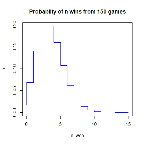
Finally, here’s a plot of the probability of winning n_won  games out of 150, with a vertical line at 7 wins:

# plot distribution
n_won <- c(0:15)
p <- c()
for(n in n_won) {
  p[n+1] <- binom_prob(n, n_played, p_win)
}
plot(n_won, p, type='S', col='blue', main='Probabilty of n wins from 150 games')
abline(v=7, col='red')

A simpler way?

You just saw the classic approach to solving what was actually a very simple problem. But if you didn’t know the formula for the binomial probability distribution, it would be hard to know where to start. It’s also very easy to get tripped up with p-values and their confusing double-negative terminology. I think you can probably see some evidence for my claim that we can easily end up forgetting the question we were trying to answer in the first place! And this was a very simple problem – things get much worse from here.

The good news is, there’s an easier way. We could watch someone play 150 games of roulette, then write down the number of games they won. We could then watch another 150 games and write down that result. If we did this many times, we would be able to plot a histogram showing the frequency of each result. If we watched many sequences of 150 games, we could expect the observed frequencies to start approaching the true frequencies.

But who has time to watch a few thousand sequences of 150 roulette games? Better to leverage our programming skills and simulate a few thousand such sequences.

Here’s a really simple roulette simulator that simulates sequences of roulette games, and returns the number of winning games in each sequence. We can use this simulator to generate sound statistical insights about our gambler.

The great thing about this simulator is that you can build it just by knowing a little about the game of roulette – it doesn’t matter if you’ve never heard of the binomial probability function, you can use the simulator to get robust answers to statistical questions.

# roulette simulator
roulette_sim <- function(num_sequences, num_games) {
  lucky_number <- 12
  games_won_per_sequence <- c()
  for(n in c(1:num_sequences)) {
    spins <- sample(0:36, num_games, replace=TRUE)
    games_won_per_sequence[n] <- sum(spins==lucky_number)
  }
  return(games_won_per_sequence)
}

Most of the work is being done in the line spins <- sample(0:36, num_games, replace=TRUE)  which we are using to simulate a single sequence of num_games  spins of the roulette wheel. The sample()  function randomly selects numbers between 0 and 36 num_games  times and stores the results in the spins  variable. Then, the line games_won_per_sequence[n] <- sum(spins==lucky_number)  calculates the number of spins in the sequence that came up with our lucky_number  and stores the result in the vector games_won_per_sequence . I used the number 12 as the lucky_number  parameter, which is what I would choose if I were forced to choose a lucky number, but any number in the range 0:36 will do, as they all have an equal likelihood of turning up in any given “spin”.

Let’s simulate 10,000 sequences of 150 games and plot the result in a histogram. Simply do:

# plot histogram of simulated 150-game sequences
hist(roulette_sim(10000, 150), col='blue')

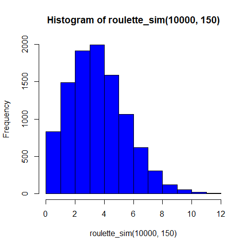
And you’ll end up with a histogram of games won that looks like this:4Results will differ slightly each time you run the simulation.

Hmmm…the shape of our histogram looks very much like the shape of the binomial distribution that we plotted above using the classic approach. Interesting! Could it be that our simulation is indeed a decent representation of reality?

We can also calculate an empirical p-value from our simulation results by calculating the proportion of times we won at least seven games. Here’s a general function for calculating the empirical p-value, and an example of using it to calculate our gambler’s p-value:

sim_pval <- function(num_sequences, num_games, val) {
  games_won_per_sequence <- roulette_sim(num_sequences, num_games)
  return(sum(games_won_per_sequence >= val)/num_sequences)
}
pval <- sim_pval(10000, 150, 7)

When I ran this code, I got a p-value of 11.3, compared with a p-value of 11.4 calculated above using the classic approach. You’ll get a slightly different result every time you run this code, but the more sequences you simulate (the num_sequences  parameter), the more the empirical result will converge to the theoretical one.

Initial Conclusion on Practical Statistics

My intent with this article was to convince you that you can get statistically sound insights without resorting to the complexities of classic statistics.  Personally, I find myself going around in circles and expending great energy for little reward when I try to solve a problem with the classic approach. On the other hand, I find that I get real insights and real intuition into a problem through simulation.

Simulation, however, is just one way you can hack statistics, and it won’t be applicable in all situations. For instance, in this example we happen to have a precise generative model for the phenomenon we wish to explore – namely, the probability of winning a game of roulette. In most trading situations, we normally have only data or at best some assumptions about the underlying generative model.

Read part 2 of this series – Practical Statistics: The Law of Large Numbers

Afterthought

Apparently Thorp and Shannon’s roulette computer could predict which octant of the wheel the ball would end up in. That means that they could reduce the possible outcomes to five numbers of the thirty-seven total possibilities, increasing their odds of winning from 1/37 to 1/5. That means that from a sequence of 150 games, Thorp and Shannon might expect to win a staggering 30 times.

If we simulate the probability of Thorp and Shannon winning 30 of 150 games of roulette by chance:

# p-value for Thorp and Shannon
pval <- sim_pval(10000, 150, 30)

we end up with a p-value of zero! That is, there is no conceivable possibility of winning 30 of 150 games of roulette by chance alone. In reality, of course the real probability isn’t zero, but apparently 10,000 simulations isn’t enough to detect a single occurrence of this many wins! Resorting to the analytical solution,

# analytical p-value for Thorp and Shannon
pval <- binom_pval(30, 150, 1./37)

we find that the probability of 30 winning spins from 150 is 1.2e-17!

So how did Thorp and Shannon evade detection? Can we assume that the pit bosses back in the 1960s weren’t concerning themselves with the possibility that someone might be cheating? Actually, if you read their story, you find that Thorp and Shannon were plagued by the vagaries of the device itself, dealing with constant breakdowns and malfunctions that limited their ability to really exploit their edge.

Still, it’s a brilliant story and you really have to admire their ingenuity, not to mention their guts in taking on the casinos at their own game.