
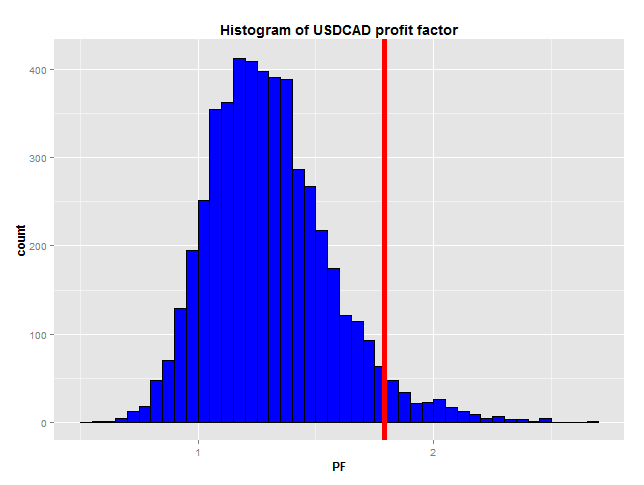
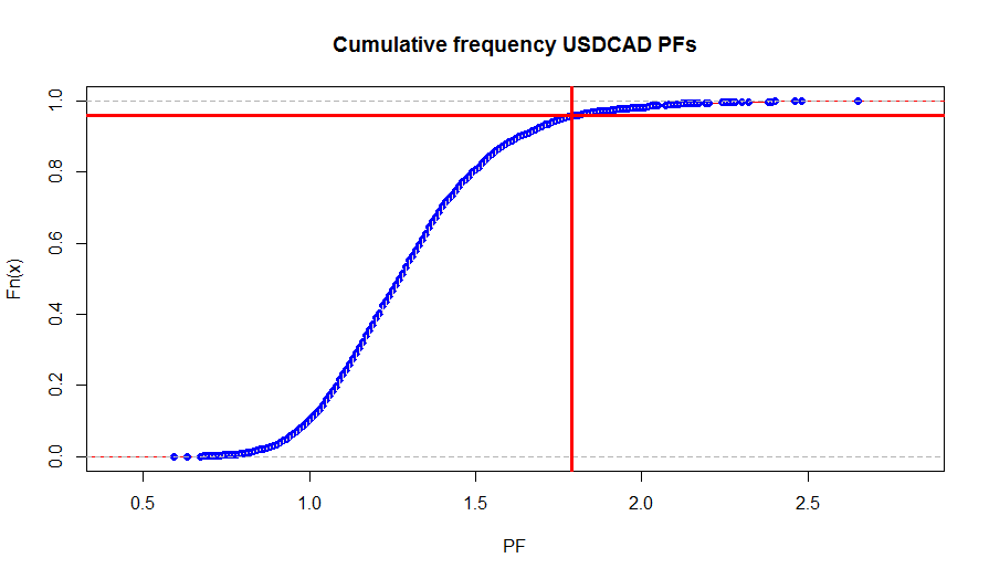
 As expected, the profit factors are generally normally distributed with some skewness. Our USD/CAD portfolio component did well in the out of sample backtest, with a profit factor of 1.79. The profit factor distribution obtained by simulating random trades of the dame direction and average frequency and duration is right skewed, indicating a trend in the same direction as our strategy – short in this case. This may indicate that some of the non-random strategy’s performance is due to the market’s trend, or put another way, due to simply being lucky enough to be in the right market at the right time. Examination of the cumulative frequency distribution reveals that our non-random strategy out-performed 96% of random strategies. So we can conclude with 96% certainty that our strategy has predictive power, even though it trades with the dominant trend in the market. Put another way, we are 96% certain that the strategy’s performance was not just due to being in the right market at the right time. I am comfortable trading this component in my live portfolio.
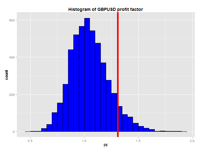
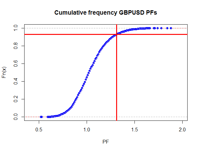 Similar examination of the GBP/USD portfolio component reveals a slight right skew in the random profit factor distribution, indicating a slight trend in the same direction as the candidate strategy trades. In this case, the candidate strategy out performed 92.5% of random strategies. This candidate lies in a tricky position on the distribution: an oft-cited minimum confidence limit in the scientific literature is the 95th percentile, of which this strategy is just shy. In addition, its out of sample profit factor was only 1.20, which is on the low side. All things considered, I’ll leave this component out of my active portfolio.
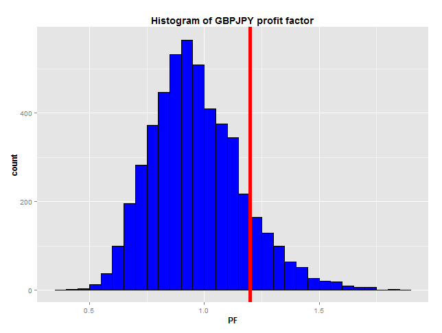
 Finally, examination of the GBP/JPY data reveals a left skew in the distribution of the random trader’s profit factor, indicating a slight trend in the opposite direction to the candidate strategy. In this case, our non-random strategy’s profit factor of 1.31 beats 89% of random traders. Again, I’m not overly comfortable adding this strategy to my live portfolio, however the fact that it does reasonably well even while trading against the underlying bias in the price data is enough to pique my interest. I’m going to add this component to my live forward test account, which is only minimally capitalised, but is a much more accurate indicator of performance than a demo account. I’ll monitor this component on that account for some time, perhaps two or three months, gathering further statistics about its performance. Depending on the results, I may add it to my live portfolio, or I may discard it altogether. I don’t know enough at present to make a decision one way or another.
Would you make the same decisions I made in assessing these candidate strategies? If not, why not?
Finally, examination of the GBP/JPY data reveals a left skew in the distribution of the random trader’s profit factor, indicating a slight trend in the opposite direction to the candidate strategy. In this case, our non-random strategy’s profit factor of 1.31 beats 89% of random traders. Again, I’m not overly comfortable adding this strategy to my live portfolio, however the fact that it does reasonably well even while trading against the underlying bias in the price data is enough to pique my interest. I’m going to add this component to my live forward test account, which is only minimally capitalised, but is a much more accurate indicator of performance than a demo account. I’ll monitor this component on that account for some time, perhaps two or three months, gathering further statistics about its performance. Depending on the results, I may add it to my live portfolio, or I may discard it altogether. I don’t know enough at present to make a decision one way or another.
Would you make the same decisions I made in assessing these candidate strategies? If not, why not?
Free Case Study:
A wantaway engineer’s journey into professional trading and out again
I went from engineering to an equity partnership at a prop trading firm to running my own systematic trading operation from home in Western Australia.
This case study is the full story – every mistake, every breakthrough, and some things I trade today.


Why are you only using profit factor to evaluate whether or not your strategy has predictive power over random strategies? Would you not want to look at other variables too?
Possibly – although I’m struggling to think of such a case. Depending on the circumstances, there may be a number of performance metrics that may be of interest. But the purpose here is simply to show whether a strategy is better than random, not to evaluate the strategy from multiple perspectives (that comes later). In order to do that, I don’t need a raft of other performance metrics – I only need one, and something simple will do the trick. Profit factor is easy to implement and is directly comparable between markets and systems. It is useful for the intended purpose, but if you prefer a different metric, go ahead and use it. Just be aware that the purpose here is not a thorough evaluation of the strategy, its simply to decide whether it is significantly better than random.