Shannon Entropy: A Genius Gambler’s Guide to Market Randomness

Before you commit your precious time to read this post on Shannon Entropy, I need to warn you that this is one of those posts that market nerds like myself will get a kick out of, but which probably won’t add much of practical value to your trading.

The purpose of this post is to scratch the surface of the markets from an information theoretic perspective, using tools developed by none other than the father of the digital age, Claude Shannon. Specifically, we’re going to tinker with the concept of Shannon Entropy.

Shannon (the man, not the entropy) was one of those annoying people that excels at everything he touches. Most notably, he was the first to describe the theory of electrical circuit design (in his Master’s thesis at the age of 21, no less). Later, around 1948, he discovered Information Theory, which leverages his unique-at-the-time understanding that computers could express numbers, words, pictures, even audio and video as strings of binary digits.

Not being one to let his genius go to waste, he and his buddy Ed Thorpe secretly used wearable computers to beat roulette in Vegas casinos by synchronising their computers with the spins of the wheel. They also beat the casinos by counting cards at Blackjack.

Between Information Theory and digital circuit design (and less so his gambling escapades), Shannon’s work essentially ushered in the digital world we find ourselves in today.

What is Shannon Entropy?

Measured in bits, Shannon Entropy is a measure of the information content of data, where information content refers more to what the data could contain, as opposed to what it does contain. In this context, information content is really about quantifying predictability, or conversely, randomness.

This concept of information is somewhat counter-intuitive. In everyday usage, we equate the word information with meaning. Information has some meaning, otherwise it’s not really information. In Shannon’s Information Theory, information relates to the effort or cost to describe some variable, and Shannon Entropy is the minimum number of bits that are needed to do so, on average.

This sounds a bit whacky, but will become clearer as we introduce some equations and examples. The key is to divorce the information theoretical definition of information from our everyday concept of meaning.

Illustrating the Concept of Shannon Entropy

Say we have some random variable, like a coin toss. Your friend tosses the coin and hides the result from you. You can discern the outcome of any individual coin toss by asking just one binary (yes-no) question: was the outcome a head ?1Equally, we can ask whether it was a tail and still end up with the same knowledge.

The number of binary questions we need to ask to describe each outcome is one. Here and in the examples below, consider that ‘the cost of encapsulating information’ is analogous to ‘the number of questions required to describe a random variable’.

Next, consider a deck of cards with the jokers removed. Our friend shuffles the deck, draws a card and records its suit without showing us. Our friend then replaces the card, reshuffles the deck and repeats. Our friend’s record of the suits drawn from the deck is then a random variable with four equally probable outcomes. What is the minimum number of binary questions we must now ask, on average, to ascertain the suit of each draw?

Our first question could be is the suit red? Then, if the answer was yes, we might ask is the suit a diamond?  Otherwise, we might ask is the suit a spade? If you think about it, regardless of the suit and the binary questions asked, we always need two questions to arrive at the correct answer.

Now consider a deck stacked with one suit and with some cards of the other suits removed. Say we have 26 hearts, 10 diamonds, 8 spades and 8 clubs. The outcome of a card draw is no longer completely random in the sense that the outcomes are no longer equally likely. We can use that knowledge to reduce the number of questions we need, on average, to arrive at the correct suit.

The probability of a card being a heart, diamond, spade or club is now 0.5, 0.19, 0.15 and 0.15 respectively. If our first question is Is the suit a heart? in 50% of cases, we will have arrived at the correct suit after a single question. If the answer is No, our next question would be Is the suit a diamond? Now, in almost 70% of cases, we will have our answer within two questions. In 30% of cases, we’ll need a third question.

Now, the average number of questions is simply the sum of the probabilities associated with each possible number of questions, that is

[\frac{26}{52} * 1 + \frac{10}{52} * 2 + \frac{8+8}{52}*3  \approx 1.81]

Recall that when all suits had an equal probability of occurrence, we always needed to ask two questions to ascertain any particular draw’s suit. This equal weight case corresponds to the system that maximizes randomness and minimizes order. When we add some order to the system by making one outcome more likely, we reduce the average number of questions to ascertain the suit, in this case to 1.81.2How can you have 1.81 questions? Remember that this is an average value. Sometimes you only need one question, sometimes you need 2, and sometimes 3. But on average, you need only 1 more often than you need 2 or 3.

Defining Shannon Entropy

The phenomenon we’ve just seen is analogous to Shannon Entropy, which measures the cost or effort required to describe a variable. Like the number of questions we need to arrive at the correct suit, Shannon Entropy decreases when order is imposed on a system and increases when the system is more random. Entropy is maximized (and predictability minimized) when all outcomes are equally likely.

Shannon Entropy, (H) is given by the following equation:

[H = -\sum_{i=1}^np_i\log_2 p_i]

Where (n) is the number of possible outcomes, and (p_i) is the probability of the (i^{th}) outcome occurring.

Why did Shannon choose to use the logarithm in his equation? Surely there are more intuitive ways to measure information and randomness? Certainly when I first looked at this equation, I wondered where it came from. It turns out that randomness is a tricky thing to quantify, and there are several approaches in addition to Shannon’s. The choice of measure is really informed by the properties we wish our measure to take on, rather than the properties of the phenomenon being measured. In this case, it is partially to do with how we might perceive the measure of information to change (for example, to double the number of possible states of a binary string, we simply add a bit, which is equivalent to incrementing the base 2 logarithm of the number of possible states).

More than that, using the logarithm also means that a very likely outcome does not contribute much to the randomness measure (since in this case the (log_2 p_i) term approaches zero), and that a very unlikely outcome also does not contribute much (since in this case the (p_i) term approaches zero). In addition, the additive property of logarithms simplifies combining entropies from different systems.

Shannon Entropy in Zorro

Zorro implements a Shannon Entropy indicator, but it’s tucked away in the Indicators section of the manual, one of dozens of functions listed on that page, and it’s easy to miss it.

Zorro’s is quite a clever implementation that works by converting a price curve into binary information: either the current value is higher than the previous one, or it is not. The function then detects and counts every combination of price changes in the curve of a given length. For example, we can check for patterns of two consecutive price changes, of which there are four possible binary combinations (up-up, down-down, up-down, down-up). Zorro then determines the relative frequency of these binary combinations, which are of course the empirically determined (p) values for use in the Shannon Entropy equation.

Once the (p)’s are known, Zorro simply implements the Shannon Entropy equation and returns the calculated value for (H), in bits. That means that the maximum (H), which corresponds to a perfectly random system, is equal to the pattern size. In our example of analyzing patterns of length 2, (H = 2) implies that all the patterns were equally likely to occur, and thus the system is purely random.

Of course, deviations from randomness are of interest to traders, because less randomness implies more predictability.

Before we dive into some examples, let’s take a look at the arguments of the ShannonEntropy()  function:

1. The function’s first argument is a data series, usually a price curve. Remember, the function differences this series for us so we can simply supply raw prices.
2. Next, we supply an integer time period over which to analyze the price curve for randomness.
3. Finally, we supply the length of the patterns that we are interested in, from 2 to 8, remembering that there are \(2^x\) possible patterns, where \(x\) is the pattern length.

Here’s a simple implementation that plots the Shannon Entropy for the SPY ETF from 2000 to 2016 for all pattern sizes from 2 to 5 measured at the daily time scale (the script gets its data from the Alpha Vantage API; if you don’t have access,  comment out lines 16-17 and select an asset from your Zorro GUI):

/* SHANNON ENTROPY

*/

function run()
{
    set(PLOTNOW);
    StartDate = 2000;
    EndDate = 2016;
    BarPeriod = 1440;
    LookBack = 80;
    PlotHeight1 = 250;
    PlotHeight2 = 125;
    PlotWidth = 800;
    
    if(is(INITRUN)) assetHistory("SPY", FROM_AV);
    asset("SPY");
    
    int period = LookBack;
    vars Closes = series((priceClose()));   
    int patterns;
    for(patterns=2;patterns<=5;patterns++)
    {
        var H = ShannonEntropy(Closes, period, patterns);
        plot(strf("H_%d", patterns), H, NEW|BARS, BLUE);
    }
}

And the resulting plot:

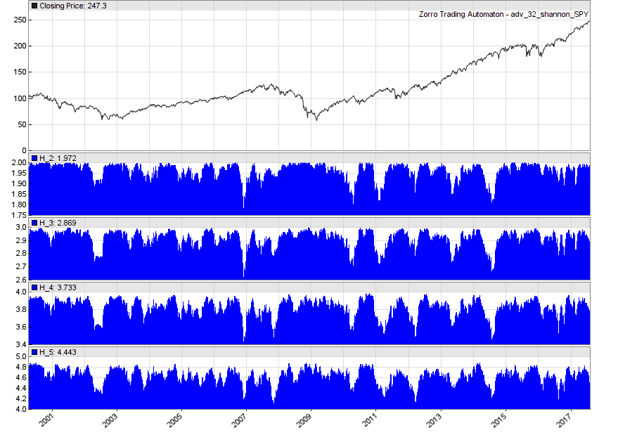While the markets are clearly highly random, we can see regular departures from perfect randomness across multiple pattern sizes. That’s good news! If the markets aren’t completely random, then there is hope for us traders!

The next obvious question is how could we apply this measure of randomness in our trading? In reality, you’re unlikely to derive a trading strategy from the calculation of (H) in isolation (more on this below), but perhaps there is merit in applying it as an additional trade filter. For example, if you’ve found an edge in a particular market, perhaps it makes sense to apply it selectively during periods of predictability. Like all backwards-looking measures however, we need to consider that the past may not be like the future, and we need to be careful about optimizing the lookback period used in our analysis.

The Principle of Maximum Entropy

While the past may not be like the future, there is a principle related to entropy that may provide clues about the future state of a system. This principle states that complex systems tend to evolve so as to maximize entropy production under present constraints. This principle of maximum entropy has found application in physics, biology, statistics and other fields. Perhaps we can apply it to the markets too.

If the principle of maximum entropy does indeed apply to the markets, we would expect that given an existent series of price changes, the next value in the series should tend to maximize the entropy of the system. That means that if we know the market direction that maximizes its entropy, we have a clue as to which way the market is more likely to move. To test this, we can simulate possible future price movements and work out which scenarios tend to maximize the system’s entropy at any given time.

Below is some code to accomplish this. Firstly, we need to set the PEEK  flag (line 8), which enables the price()  functions to access future data. We calculate Shannon Entropy of our price series as before (lines 30-31). But this time, we need to create two additional arrays that correspond to the two possible entropy states at the next time period (line 19). That is, one array corresponds to an up move, and the other corresponds to a down move. We fill these arrays in a for()  loop where we copy across the existing series into our new arrays, starting from index 1 (lines 21-25). Then, we place either a higher or lower price compared to the current price at index 0 of each array (lines 26-27).

Now we’ve got arrays from which we can calculate the two possible entropy states at the next time period (remember that entropy is calculated from binary price patterns, therefore only the direction of the next move is important, not its magnitude). Then, we simply calculate the entropy of both states, and the one that returns the higher value is our prediction (lines 30-31).

I’m going to apply this idea to one of the most efficient (and therefore random) markets around: the foreign exchange markets. Rather than run a traditional backtest, in this case I just want to count the number of correct and incorrect forecasts made by our maximum entropy predictor, and sum the total number of pips that would be collected in the absence of the realities of trading (slippage, commission and the like). Lines 33-41 accomplish this.

Here’s the code:

/* SHANNON ENTROPY

*/


function run()
{
    set(PLOTNOW|PEEK);
    StartDate = 2004;
    EndDate = 2016;
    BarPeriod = 1;
    LookBack = 100;
    
    int patterns = 2;
    int period = LookBack;
    vars Closes = series((priceClose()));       
    
    // create possible future entropy states
    var up[501], down[501]; //set these large to enable experimenting with lookback - can't be set by variable
    int i;
    for(i=1;i<period+1;i++)
    {
        up[i] = Closes[i];
        down[i] = Closes[i];    
    }
    up[0] = Closes[0] + 1;
    down[0] = Closes[0] - 1;
    
    // get entropy of next state
    var entropyUp = ShannonEntropy(up, period+1, patterns);
    var entropyDn = ShannonEntropy(down, period+1, patterns);   
    
    // idealized backtest
    static int win, loss;
    static var winTot, lossTot;
    if(is(INITRUN)) win = loss = winTot = lossTot = 0;
    
    if(entropyUp > entropyDn and priceClose(-1) > priceClose(0)) {win++; winTot+=priceClose(-1)-priceClose(0);}
    else if(entropyUp < entropyDn and priceClose(-1) < priceClose(0)) {win++; winTot+=priceClose(0)-priceClose(-1);}
    else if(entropyUp > entropyDn and priceClose(-1) < priceClose(0)) {loss++; lossTot+=priceClose(0)-priceClose(-1);}
    else if(entropyUp < entropyDn and priceClose(-1) > priceClose(0)) {loss++; lossTot+=priceClose(-1)-priceClose(0);}
        
    if(is(EXITRUN))
        printf("\n\n%W: %.2f%%\nWins: %d Losses: %d\nWinTot: %.0f LossTot: %.2f\nPips/Trade: %.1f", 
        100.*win/(win + loss), win, loss, winTot/PIP, lossTot/PIP, (winTot-lossTot)/PIP/(win+loss));
    
    ColorUp = ColorDn = 0;
    plot("PipsWon", (winTot-lossTot)/PIP, MAIN|BARS, BLUE);
    PlotWidth = 1000;
}

You can have some fun experimenting with this script. Try some different assets, different bar periods and different pattern sizes. You’ll see some interesting things in relation to randomness – some of which may go against the existing common wisdom.

As an example, when we run this script using 1-minute bars, we nearly always get a very slightly positive result, usually on the order of 51% correct predictions. The plot of pips collected for the major currency pairs from 2004-2016 are shown below (from left to right, top to bottom, AUD/USD, USD/JPY, USD/CAD, EUR/USD, NZD/USD, GBP/USD):

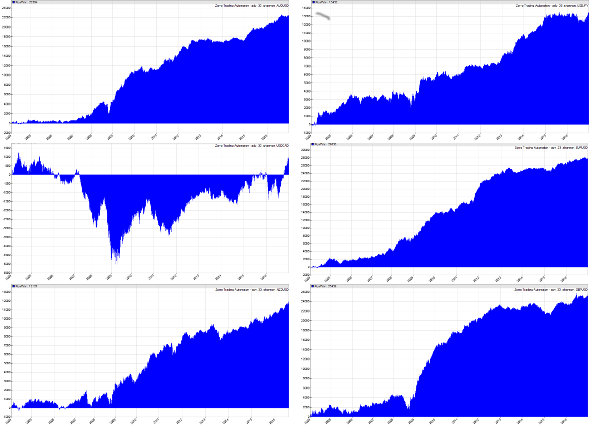While there is very likely a tiny edge here, it is just that: tiny. In reality, you’ll never make money by predicting the direction of the next minute’s price change correctly 51% of the time! However, what if you could predict the direction over a longer time frame and improve the accuracy of your prediction? Could you make money from that?

Here’s an idea for extending our directional forecast based on maximum entropy to two time steps into the future. Now we have four possible scenarios (up-up, down-down, up-down, down-up) to assess. In the idealized backtester, we now go long when the two-ahead entropy is maximized by the up-up case, and short when it is maximized by the down-down case.

/* SHANNON MULTI-STEP AHEAD FORECAST

*/

function run()
{
    set(PLOTNOW|PEEK);
    StartDate = 2010;
    EndDate = 2019;
    BarPeriod = 1;
    LookBack = 100;

    int patterns = 3;
    int period = LookBack;
    vars Closes = series((priceClose()));   

    var upup[501], dndn[501], updn[501], dnup[501];
    int i;
    for(i=1;i<period+1;i++)
    {
        upup[i] = Closes[i];
        dndn[i] = Closes[i];
        updn[i] = Closes[i];
        dnup[i] = Closes[i];    
    }
    upup[1] = Closes[0] + 1;
    upup[0] = upup[1] + 1;
    dndn[1] = Closes[0] - 1;
    dndn[0] = dndn[1] - 1;
    updn[1] = Closes[0] + 1;
    updn[0] = updn[1] - 1;
    dnup[1] = Closes[0] - 1;
    dnup[0] = dnup[1] + 1;
    
    var entropyUpUp = ShannonEntropy(upup, period+2, patterns);
    var entropyDnDn = ShannonEntropy(dndn, period+2, patterns);
    var entropyUpDn = ShannonEntropy(updn, period+2, patterns);
    var entropyDnUp = ShannonEntropy(dnup, period+2, patterns);
    
    static int win, loss;
    static var winTot, lossTot;
    if(is(INITRUN)) win = loss = winTot = lossTot = 0;
        
    if(max(max(max(entropyUpUp, entropyDnDn), entropyUpDn), entropyDnUp) == entropyUpUp and priceClose(-2) > priceClose(0)) {win++; winTot+=priceClose(-2)-priceClose(0);}
    else if(max(max(max(entropyUpUp, entropyDnDn), entropyUpDn), entropyDnUp) == entropyDnDn and priceClose(-2) < priceClose(0)) {win++; winTot+=priceClose(0)-priceClose(-2);}
    else if(max(max(max(entropyUpUp, entropyDnDn), entropyUpDn), entropyDnUp) == entropyUpUp and priceClose(-2) < priceClose(0)) {loss++; lossTot+=priceClose(0)-priceClose(-2);}
    else if(max(max(max(entropyUpUp, entropyDnDn), entropyUpDn), entropyDnUp) == entropyDnDn and priceClose(-2) > priceClose(0)) {loss++; lossTot+=priceClose(-2)-priceClose(0);}

    if(is(EXITRUN)) printf("\n\n%W: %.2f%%\nWins: %d Losses: %d\nWinTot: %.0f LossTot: %.0f\nPips/Trade: %.1f", 100.*win/(win + loss), win, loss, winTot/PIP, lossTot/PIP, (winTot-lossTot)/PIP/(win+loss));
    
    ColorUp = ColorDn = 0;
    plot("pips", (winTot-lossTot)/PIP, MAIN|BARS, BLUE);
    PlotWidth = 1000;
    
}

And here’s a plot of the number of pips collected over the past few years, excluding trading frictions, on EUR/USD:

Conclusions

In this post, we looked at the markets from a slightly different perspective, through the lens of Information Theory. In particular, we saw how Shannon Entropy is a measure of the degree of order or predictability within a system, with increasing entropy corresponding to more randomness and maximum entropy occurring when all outcomes are equally likely. We saw that financial markets are highly random (in general displaying a Shannon Entropy close to that of a perfectly random system), but that they do depart from randomness regularly. They may even do so differently depending on the time horizon and granularity over which they are analyzed.

We also saw an attempt to use Shannon Entropy in a standalone trading system via the principle of maximum entropy production. While such a system does appear to have a small edge, in reality, it will be difficult to make a consistent trading system from these predictions alone as transaction costs will usually swamp the edge.

While this is all very interesting from an academic perspective, if you can think of a practical application to trading, we’d love to hear about it in the comments.