Revenge of the Stock Pickers

To say we’re living through extraordinary times would be an understatement.

We saw the best part of 40% wiped off stock indexes in a matter of weeks, unprecedented co-ordinated central bank intervention on a global scale, and an unfolding health crisis that for many has already turned into a tragedy.

As an investor or trader, what do you do?

You manage your exposures the best you can, dial everything down, and go hunting for the opportunities that inevitably present themselves in a stressed out market.

We’ve been hunting pretty much since this thing kicked off – and we want to show you what we found. And, more importantly, the tools and approach we used to find them.

To that end, we are opening the gates to our Robot Wealth Pro community, a tight-knit network of independent traders with whom we share our firm’s research, data, systematic trading strategies, and real-time ideas.

We normally insist that you go through an introductory Bootcamp before joining our Pro team, but these are extraordinary times and we want to get after these opportunities as soon as possible. If you’re interested in joining us, go here for more information.

We have a ton of ideas, strategies, and tactics for not only surviving the current sell-off in risk assets, but also to profit. I’ll share one in this post.

Last year, some folks at a Baltimore investment management firm published a paper with the catchy title Revenge of the Stock Pickers. The gist of the paper is as follows:

When an ETF sells off on high volume, correlations among its constituents tend to increase, often quite significantly. During normal times, some constituents have lower beta to the ETF than others, but during significant sell-offs, these low-beta constituents get dragged down along with the ETF, regardless of their own idiosyncratic exposure to whatever caused the sell-off. The authors hypothesise that such throwing the baby out with the bathwater can lead to temporary mispricings upon which stock pickers can capitalise.

With the inexorable rise of passive investing, this certainly seems a plausible hypothesis at first glance. Given the current state of things, we decided to dig a little deeper and find out if there’s anything to the theory.

Turns out there is. 

Our game plan for tackling this will be:

• Get some ETF historical price data – both for the ETF and its constituents
• Look at correlations between constituents during normal times and stressed times
• Calculate historical returns to low- and high-beta constituents and figure out if we have some alpha on our hands
• Suggest a simple trading strategy

ETF data

We like to start simple, so to kick things off we’ll look at the SPDR sector ETFs. We’ll look at the following sectors:

• Materials (XLB)
• Energy (XLE)
• Financials (XLF)
• Industrials (XLI)
• Technology (XLK)
• Staples (XLP)
• Utilities (XLU)
• Health care (XLV)
• Consumer discretionary (XLY)

Here’s some Python code for downloading the constituents of each ETF to separate CSV files:

"""download to csv file ETF holdings"""

import pandas as pd


def get_holdings(spdr_ticker):
    
    url = f'http://www.sectorspdr.com/sectorspdr/IDCO.Client.Spdrs.Holdings/Export/ExportCsv?symbol={spdr_ticker}'
    df = pd.read_csv(url, skiprows=1).to_csv(f'{spdr_ticker}_holdings.csv', index=False)
        
    return df
    
    
if __name__ == "__main__":
    
    tickers = ['XLB', 'XLE', 'XLF', 'XLI', 'XLK', 'XLP', 'XLU', 'XLV', 'XLY']
    
    for t in tickers:
        get_holdings(t)

We’ll also need historical market data for the ETFs and their constituents. I’ll be using our Robot Wealth Pro database of market data for this.

We need some way to identify high-volume sell-offs, so let’s create rolling means and standard deviation of volumes, and then a rolling z-score of volume for each ETF. The tidyquant R package is great for this sort of thing:

library(tidyverse)
library(tidyquant)

source("./robotwealth_tools.R")

# load stock-level prices
load(paste0(STOCK_FOLDER, 'raw-data.RData'))

# load etf prices
etfs <- c('XLB', 'XLE', 'XLF', 'XLI', 'XLK', 'XLP', 'XLU', 'XLV', 'XLY')
etf_prices <- get_daily_OHLC(etfs, ETF_FOLDER)

# calculate returns
etf_returns <-  etf_prices %>%
  group_by(ticker) %>%
  mutate(returns = log(close) - log(lag(close))) %>%
  na.omit()

wdw <- 250
etf_returns <- etf_returns %>%
  group_by(ticker) %>%
  tq_mutate(select = volume, mutate_fun = rollapply, width = wdw, align = "right", FUN = mean, na.rm = TRUE, col_rename = "vol_mean") %>% 
  tq_mutate(select = volume, mutate_fun = rollapply, width = wdw, align = "right", FUN = sd, na.rm = TRUE,   col_rename = "vol_sd") %>% 
  mutate(zscore = (volume - vol_mean) / vol_sd)

# Plot volume and it's moving average by ticker
etf_returns %>%
  na.omit() %>%
  ggplot(aes(x = date, y = volume)) +
   geom_line() + 
   geom_line(aes(y = vol_mean), color='red') +
   facet_wrap(~ticker)

# plot zscores of volume
etf_returns %>% 
  na.omit() %>%
  ggplot(aes(x = date, y = zscore)) +
    geom_line() +
    facet_wrap(~ticker)

There seem to be enough volume spikes for us to do some analysis.

ETF constituent correlations

First, let’s see if the idea that ETF constituent correlations increase during times of stress. In the spirit of keeping things simple, we’ll plot some heatmaps of correlation calculated:

• Over the whole data set
• On high volume days only

Let’s look at the Financials ETF, XLF.

get_constituents <- function(etf) {
  constituents <- read.csv(paste0('./', etf, '_holdings.csv'), stringsAsFactors = FALSE)
  constituents <- constituents %>%
    select(Symbol) %>%
    pull()
  
  return(constituents)
}

# get etf constituents
etf <- 'XLF'
etf_constituents <- get_constituents(etf)

# make dataframe of constituent prices
constituent_prices <- prices_df %>%
  filter(ticker %in% etf_constituents)

# calculate returns
constituent_returns <-  constituent_prices %>%
  group_by(ticker) %>%
  mutate(returns = log(close) - log(lag(close))) %>%
  select(date, ticker, returns) %>%
  na.omit()

library(corrplot, quietly = TRUE)

# pairwise correlation of constituents using as much data as possible (different number of observatiosn for different pairs)
corr_complete_pairwise <- constituent_returns %>%
  spread(key = ticker, value = returns) %>%
  select(-date) %>%
  cor(use = "pairwise.complete.obs", method='pearson')

corrplot(corr_complete_pairwise)

# pairwise correlation on days when zscore of volume is > 3

# high etf vol days
high_vol_days <- etf_returns %>% 
  filter(zscore >= 3) %>%
  ungroup() %>%
  filter(ticker == etf) %>%
  select(date) %>%
  pull()

# pairwise correlation of constituents using as much data as possible (different number of observatiosn for different pairs)
corr_complete_pairwise_high_vol <- constituent_returns %>%
  filter(date %in% high_vol_days) %>%
  spread(key = ticker, value = returns) %>%
  select(-date) %>%
  cor(use = "pairwise.complete.obs", method='pearson')

corrplot(corr_complete_pairwise_high_vol)

Here’s the correlation of the XLF constituents over the full data set:

Darker blue indicates higher correlation.

Here’s the same plot but now only calculated on days where the zscore of traded volume was greater than three:

We see a lot more dark blue. This tells us that, on average, correlations are higher on days where the ETF traded a high volume.

This is a very interesting result, which gives us confidence in the validity of this idea.

Returns to low-beta constituents

Now we want to look at returns of stocks wit low or high betas to the industry ETF. Do they appear to differ significantly?

In doing this, we need to be aware that we’re making a simplifying assumption: that the stocks currently in the ETF were also there historically.

That’s a somewhat heroic assumption. The return of the stocks that are currently in the ETF is going to be higher than the return of the ETF – because the ETF included stocks that performed poorly and were subsequently removed from the index.

For now, we can just keep that in the back of our mind while we try to figure out if there’s anything to this effect.

Here’s some code for calculating rolling 250-day betas for each constituent to the XLF ETF:

# rolling beta estimation
wdw <- 250
betas <- vector('list', nrow(wide_returns)-wdw)
for(i in (wdw):(nrow(wide_returns)-1)) {  
  
  wide_returns_subset <- wide_returns %>% 
    slice((i-wdw):(i-1)) %>%   
    select_if(~ sum(is.na(.)) < wdw/2) %>%  # some constituents weren't in the index during some periods - drop any with not much data in the period of interest
    dplyr::select(-date)
  
  models <- wide_returns_subset %>%
    map(~ lm(. ~ wide_returns_subset[[etf]]))  # [[ ]] returns a vector
  
  betas[[i]] <- models %>%
    map_df(., .f = extract_coeff) %>%
    mutate(date = wide_returns$date[i-1])
}

betas <- bind_rows(betas)
save(betas, file = paste0("./", etf, "_betas_", wdw, ".RData"))

Next, we need to:

• Sort our stocks into buckets according to the rank of their beta each day
• Figure out when we’re going to be long which stocks –  in this example we get long the lowest beta bucket of stocks the day after a sell-off of 2% or more in the ETF, accompanied by at least three standard deviations greater than the mean traded volume. and we hold for 40 days
• Calculate returns from doing this for each bucket

The code that does this is quite long, so I won’t reproduce it all here (if you do want it, let me know and I’ll stick it up on GitHub or otherwise share it – you’ll need your own data to reproduce the analysis as well).

Instead, let’s take a look at the results. Here are the cumulative returns to each of the five beta “buckets”:

This is a very nice result!

The returns to the lowest beta stocks (quantile 1) exceed those to the quantile 2 stocks, which exceed quantile 3’s return, and so on.

This gives us some tentative optimism that there really is something to the idea that low-beta ETF constituents tend to outperform following a high-volume sell-off in the ETF.

We don’t have a whole lot of data here, but if we extend the analysis to the other ETFs in our universe, we’ll have a whole lot more. Let’s do that next.

Buying low-beta across SPDR sectors

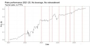
Next, we’ll run a backtest across all the SPDR sector ETFs in our universe. Again, I’ll skip the code and cut straight to the results.

For each ETF, following a down day accompanied by a three standard deviation volume spike, we:

• Buy the bottom quantile of constituents by rolling 250-day beta to the ETF
• Hold for 40 days

Here’s what that looks like:

That comes out to a Sharpe of around 0.7.

The assumptions in the backtest are that we trade at the closing price on the day of the volume spike, we trade for free, and we rebalance positions daily such that we maintain an equal dollar weight in whatever we happen to be holding.

Of course, most of those ETFs went up a lot during that period. So it’s possible these returns are simply due to the upward drift in these assets.

To assess that, let’s look at the result of doing the same thing (buying on high-volume down day and holding for 40 days) but using the ETF rather than its low-beta constituents. We expect positive performance, but lower risk-adjusted returns.

That has a Sharpe of a little under 0.3. (Again, we neglect transaction costs and rebalance daily to hold equal dollar weights in whatever ETFs we happen to be holding.)

Our active strategy had more than double the risk-adjusted returns over the backtest period. This is good evidence that we might have some alpha here.

Of course, the work is really just beginning. So far we’ve seen that:

• Correlations among ETF constituents do increase in times of stress
• Beta to the XLF ETF has been a decent factor for predicting returns conditional on a high volume sell-off
• More broadly across the SPDR sectors, buying low-beta constituents following a high-volume sell-off outperforms the broader index in risk-adjusted terms

But we also have many unanswered questions:

• What is the impact of survivorship bias on our results? (we could assess this without needing any more data by comparing the strategy returns with being long all our constituent stocks at those times)
• What about transaction costs? (this is a simple backtesting problem)
• How does this apparent alpha evolve over time? Is a 40-day hold period a sensible thing?
• How might we best capture this apparent alpha? We could:
  • implement a long-only strategy
  • use the low beta stocks as a watchlist for discretionary stock picking
  • try being long-short the low- and high-beta constituents respectively
  • long the low-beta stuff and short the ETF
• How does this play out across the vast universe of ETFs that trade today? Surely there are better opportunities than the ones we looked at first.
• In particular, broad index ETFs intuitively seem attractive given the current market context

Further, in their original paper, the authors of Revenge of the Stockpickers suggest that we can capture further alpha from this approach by also considering the context of the sell-off and whether individual stocks’ performance is justified for fundamental and macro reasons.

This strategy is just one idea that we’ll be looking at in detail in our Trading through Armageddon Bootcamp, which you can join by taking advantage of our Fasttrack to Pro offer.