Quant Signal Trade-Offs in the Real World

I want to discuss a couple of simple trade-off considerations around quant trading signals that may not be obvious.

Here’s the price of some asset:

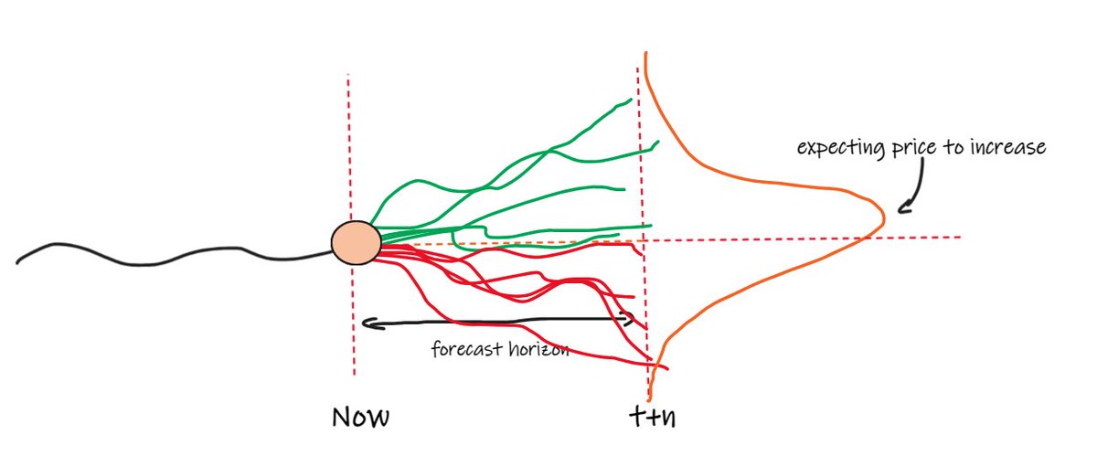
Our main job is to predict how it’s likely to move. To do this, you use information about it that you think is predictive. And at any point in time:

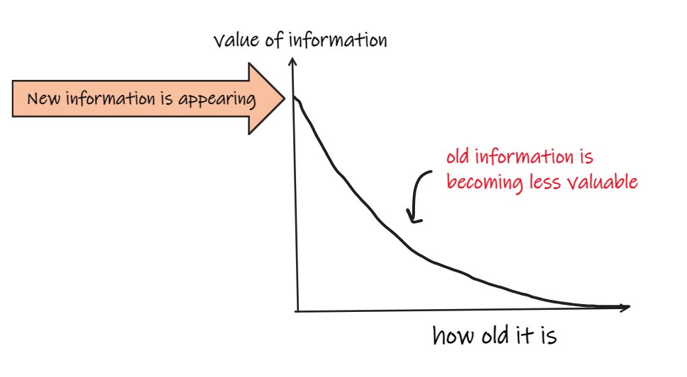
• New information is appearing (trades, quotes, events, chatter).
• Old information that used to be very important is becoming less so.

You use this information to try to create a forecast (explicit or implicit) of how you expect price to move over some future period.

To figure out if your forecast is any good, you might get a bunch of observations of your forecast and the price changes in some forward period (let’s say a minute).

Then, you might plot the subsequent returns against the forecast and, ideally, it’d look a bit like this:

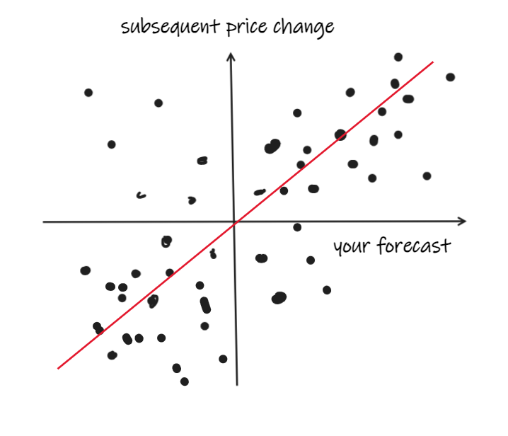
But you’ve probably got more observations than usefully fit on a scatter plot, and it’s going to look like a big old blob because market returns are super random.

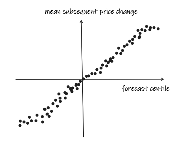
So instead, you’ll do some reduction. You might sort your observations into deciles or centiles or similar and plot mean returns.

And you may need to transform it in some way so that it’s clamped to some range, distributed in a way you understand, and doesn’t go crazy in the tails:

This is all well and good. However, being able to predict short-term returns might not be the win you think it is.

Trading is expensive, and it’s even more expensive if you are doing it when you want to (rather than someone else).

If your forecast signal looks like this, you will have a bad time:

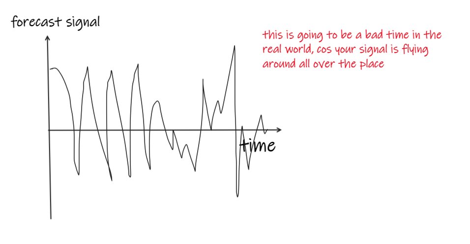
You might be really good at predicting minute-ahead returns, but you don’t actually want to turn over every minute.

You can’t afford that.

So you’d prefer your signal to be less volatile, more auto-correlated, smoother, like this:

Thus, the first trade-off is between how effective your forecast is versus how auto-correlated your signal is.

You’d prefer a smoother signal over a hyperactive, jumpy one with a slightly higher correlation to future returns.

Some things are naturally more auto-correlated (carry, rv signals). Other naturally jumpy signals can be smoothed with EWMAs and the like, which nicely model new information appearing and old information becoming slowly redundant.

We can look at this from the other direction, too.

The choice of 1 min future returns was arbitrary. We might be making trading decisions on that frequency, but we don’t intend to turn over at that frequency.

So we care about how predictive our signal is over longer horizons, too.

We might calculate the correlation of our signal with future returns over a range of other horizons. And we’d much rather this decayed slowly than quickly:

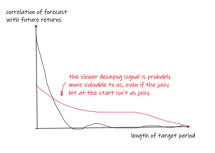
If it decays quickly, then it’s going to be very competitive to get in for the good bit. You’re going to need to be fast.

And, if we’re going to trade it successfully after costs, we’re going to have to be sat in positions with zero or very low expected return until we can get out of them cost-effectively.

So, all things being equal, we’d prefer the slightly less predictive signal that decayed more slowly.

These trade-offs are important and aren’t always easy to navigate and reason about.

Some tips:

• Plot everything – it pays to understand your signal.
• Keep everything as simple as possible, chunk big problems down, and think through things as clearly as possible.
• But also understand that, while you might chunk things down and look at them separately, the parts interact in wonderful, confusing ways.
• Use simulation to explore this as best you can.
• Thank the market gods.