Some price series are mean reverting some of the time, but it is also possible to create portfolios which are specifically constructed to have mean-reverting properties. Series that can be combined to create stationary portfolios are called cointegrating, and there are a bunch of statistical tests for this property. We’ll return to these shortly.

While you can, in theory, create mean reverting portfolios from as many instruments as you like, this post will largely focus on the simplest case: pairs trading.

What is Pairs Trading?

Pairs trading involves buying and selling a portfolio consisting of two instruments. The instruments are linked in some way, for example they might be stocks from the same business sector, currencies exposed to similar laws of supply and demand, or other instruments exposed to the same or similar risk factors. We are typically long one instrument and short the other, making a bet that the value of this long-short portfolio (the spread) has deviated from its equilibrium value and will revert back towards that value.

One of the major attractions of pairs trading is that we can achieve market neutrality, or something close to it. Because the long and short positions offset each other, pairs trading can be somewhat immune to movements of the overall market, thus eliminating or reducing market risk – theoretically at least.

Risks and Drawbacks

The fact that we can construct artificial spreads with mean-reverting properties is one of the major attractions of this style of trading. But there are some drawbacks too.

For starters, if a series was mean reverting in the past, it may not be mean reverting in the future. Constructed spreads typically mean revert when random, non-structural events affect the value of the components. A good spread combined with a good trading strategy will capture these small opportunities for profit consistently. On the other hand, when a structural shift occurs – such as a major revaluation of one asset but not the other – such a strategy will usually get burned quite badly.

How can we mitigate that risk? Predicting the breakdown of a spread is very difficult, but a sensible way to reduce the risk of this approach is to trade a diverse range of spreads. As with other types of trading, diversity tends to be your friend. I like to have an economic reason for the relationship that links the components, but to be totally honest, I’ve seen pairs trading work quite well between instruments that I couldn’t figure a relationship for. If you understand the relationship, you may be in a better position to judge when and why the spread might break down. Then again, you might not either. Breakdowns tend to happen suddenly and without a lot of warning.

Probably the best example of what not to do with a pairs trading strategy is the Long Term Capital Management meltdown. I won’t go into the details here, but there is plenty written about this incident and it makes a fascinating and informative case study.

Cointegration

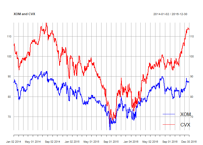
When two or more non-stationary series can be combined to make a stationary series, the component series are said to be cointegrated. One of the challenges of pairs trading is to determine the coefficients that define this stationary combination. In pairs trading, that coefficient is called the hedge ratio, and it describes the amount of instrument B to purchase or sell for every unit of instrument A. The hedge ratio can refer to a dollar value of instrument B, or the number of units of instrument B, depending on the approach taken. Here, we will largely focus on the latter approach.

The Cointegrated Augmented Dickey Fuller (CADF) test finds a hedge ratio by running a linear regression between two series, forms a spread using that hedge ratio, then tests the stationarity of that spread. In the following examples, we use some R code that runs a linear regression between the price series of Exxon Mobil and Chevron to find a hedge ratio and then tests the resulting spread for stationarity.

First, download some data, and plot the resulting price series (here we use the Robot Wealth data pipeline, which is a tool we wrote for members for efficiently getting prices and other data from a variety of sources):

# Preliminaries
library(urca)
source("data_pipeline.R")

prices <- load_data(c('XOM', 'CVX'), start='2014-01-01', end = '2017-01-01', source='av', 
                    return_data = 'Adjusted', save_indiv = TRUE)
plot(prices, col=c('blue', 'red'), main = 'XOM and CVX')
legend('bottomright', col=c('blue', 'red'), legend=c('XOM', 'CVX'), lty=1, bty='n')

Next, we create a scatter plot of our price series, which will indicate whether there is an underlying relationship between them, and fit a linear regression model using ordinary least squares:

# scatter plot of prices
plot(coredata(prices[, 'XOM.Adjusted']), coredata(prices[, 'CVX.Adjusted']), col='blue',
     xlab='XOM', ylab='CVX')

# linear regression of prices
fit <- lm(coredata(prices[, 'CVX.Adjusted']) ~ coredata(prices[, 'XOM.Adjusted']))
summary(fit)

'''
# output:

# Call:
#   lm(formula = coredata(prices[, "CVX.Adjusted"]) ~ coredata(prices[, 
#                                                                     "XOM.Adjusted"]))
# 
# Residuals:
#   Min      1Q  Median      3Q     Max 
# -9.6122 -2.2196 -0.3546  2.4747  9.3366 
# 
# Coefficients:
#   Estimate Std. Error t value Pr(>|t|)    
# (Intercept)                        -41.39747    1.88181  -22.00   <2e-16 ***
#   coredata(prices[, "XOM.Adjusted"])   1.67875    0.02309   72.71   <2e-16 ***
#   ---
#   Signif. codes:  0 ‘***’ 0.001 ‘**’ 0.01 ‘*’ 0.05 ‘.’ 0.1 ‘ ’ 1
# 
# Residual standard error: 3.865 on 754 degrees of freedom
# Multiple R-squared:  0.8752,  Adjusted R-squared:  0.875 
# F-statistic:  5287 on 1 and 754 DF,  p-value: < 2.2e-16
'''

clip(min(coredata(prices[, 'XOM.Adjusted'])), max(coredata(prices[, 'XOM.Adjusted'])),
     min(coredata(prices[, 'CVX.Adjusted'])), max(coredata(prices[, 'CVX.Adjusted'])))
abline(fit$coefficients, col='red')

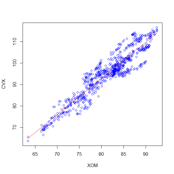The line of best fit over the whole data set has a slope of 1.68, which we’ll use as our hedge ratio. Notice however while that line is the global line of best fit, there are clusters where this line isn’t the locally best fit. We’ll likely find that points in those clusters occur close to each other in time, which implies that a dynamic hedge ratio may be useful. We’ll return to this idea later, but for now, we’ll use the slope of the global line of best fit.

Next, we construct and plot a spread using the hedge ratio we found above:

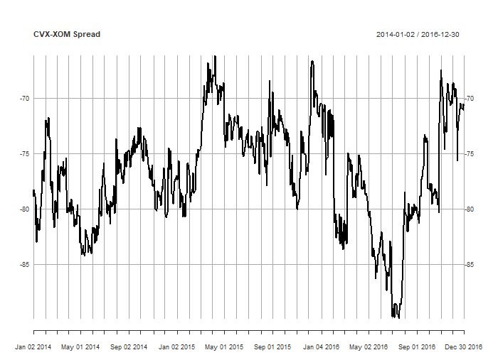
# construct and plot spread
hedge <- fit$coefficients[2]
spread <- prices[, 'CVX.Adjusted'] - hedge*coredata(prices[, 'XOM.Adjusted'])
plot(spread, main='CVX-XOM Spread', col='black')

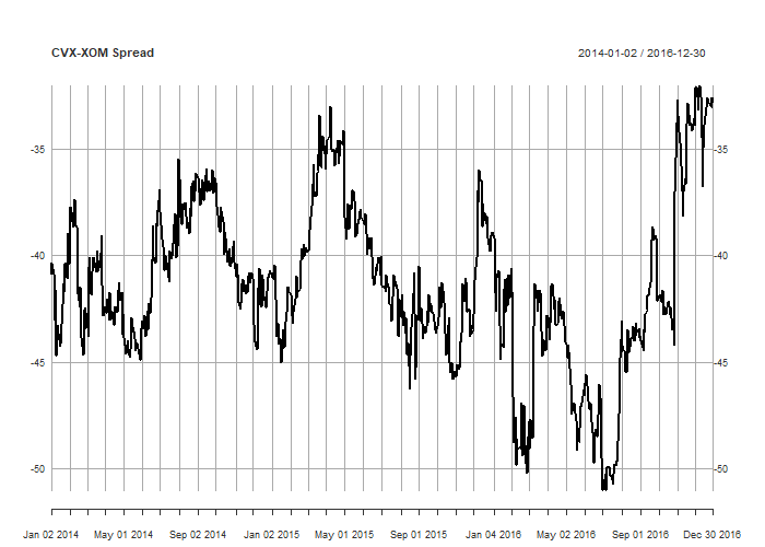The resulting spread is clearly much more mean-reverting than either of the underlying price series, but let’s test that observation using the ADF test:

# ADF TEST 
adf <- ur.df(spread, type = "drift", selectlags = 'AIC')
summary(adf)
'''
############################################### 
# Augmented Dickey-Fuller Test Unit Root Test # 
############################################### 
# 
# Test regression drift 
# 
# 
# Call:
#   lm(formula = z.diff ~ z.lag.1 + 1 + z.diff.lag)
# 
# Residuals:
#   Min      1Q  Median      3Q     Max 
# -3.8638 -0.5122  0.0037  0.5102  7.0391 
# 
# Coefficients:
#   Estimate Std. Error t value Pr(>|t|)   
# (Intercept) -1.081908   0.375640  -2.880  0.00409 **
#   z.lag.1     -0.026377   0.009032  -2.920  0.00360 **
#   z.diff.lag  -0.023002   0.036596  -0.629  0.52984   
# ---
#   Signif. codes:  0 ‘***’ 0.001 ‘**’ 0.01 ‘*’ 0.05 ‘.’ 0.1 ‘ ’ 1
# 
# Residual standard error: 0.9464 on 751 degrees of freedom
# Multiple R-squared:  0.01263, Adjusted R-squared:   0.01 
# F-statistic: 4.803 on 2 and 751 DF,  p-value: 0.008459
# 
# 
# Value of test-statistic is: -2.9204 4.3109 
# 
# Critical values for test statistics: 
#   1pct  5pct 10pct
# tau2 -3.43 -2.86 -2.57
# phi1  6.43  4.59  3.78
'''

Observe that the value of the test statistic is -2.92, which is significant at the 95% level. Thus we reject the null of a random walk and assume our series is stationary.

Implications of using ordinary least squares

You might have noticed that since we used ordinary least squares (OLS) to find our hedge ratio, we will get a different result depending on which price series we use for the dependent (y) variable, and which one we choose for the independent (x) variable. The different hedge ratios are not simply the inverse of one another, as one might reasonably and intuitively expect. When using this approach, it is a good idea to test both spreads using the ADF test and choosing the one with the most negative test statistic, as it will be the more strongly mean reverting option (at least in the past).

Another approach: total least squares

As an alternative OLS, we can use total least squares (TLS), which accounts for the variance in both series, while OLS accounts for the variance in only one (this is why we get different hedge ratios depending on our choice of dependent variable). TLS is symmetrical, and will give the same result regardless of our choice of dependent variable. In practical terms, the hedge ratios obtained by OLS and TLS usually won’t differ greatly, but when they do differ, that difference is likely to be significant. So it is worth including the TLS approach in your analysis.

Implementing TLS in R is straightforward using principal components analysis (PCA). Here’s the syntax:

# TLS for computing hedge ratio
pca <- princomp(~ coredata(prices[, 'CVX.Adjusted']) + coredata(prices[, 'XOM.Adjusted']))
tls_hedge <- pca$loadings[1, 1]/pca$loadings[2, 1]
tls_spread <- prices[, 'CVX.Adjusted'] - tls_hedge*coredata(prices[, 'XOM.Adjusted'])
plot(tls_spread, main='CVX-XOM Spread', col='black')

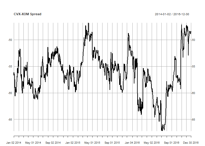The TLS approach results in a hedge ratio of 1.86 and a spread that is not all that different from our OLS hedge ratio. If we flipped the dependent and independent variables, our hedge ratio would simply the inverse of the one we just calculated.

Let’s see if it results in a more significant ADF test result:

# ADF TEST 
adf <- ur.df(tls_spread, type = "drift", selectlags = 'AIC')
summary(adf)

'''
# output
############################################### 
# Augmented Dickey-Fuller Test Unit Root Test # 
############################################### 
# 
# Test regression drift 
# 
# 
# Call:
#   lm(formula = z.diff ~ z.lag.1 + 1 + z.diff.lag)
# 
# Residuals:
#   Min      1Q  Median      3Q     Max 
# -4.0533 -0.5579  0.0100  0.5905  7.3852 
# 
# Coefficients:
#   Estimate Std. Error t value Pr(>|t|)   
# (Intercept) -1.779796   0.545639  -3.262  0.00116 **
#   z.lag.1     -0.031884   0.009693  -3.289  0.00105 **
#   z.diff.lag  -0.022874   0.036562  -0.626  0.53176   
# ---
#   Signif. codes:  0 ‘***’ 0.001 ‘**’ 0.01 ‘*’ 0.05 ‘.’ 0.1 ‘ ’ 1
# 
# Residual standard error: 1.057 on 751 degrees of freedom
# Multiple R-squared:  0.01577, Adjusted R-squared:  0.01315 
# F-statistic: 6.017 on 2 and 751 DF,  p-value: 0.002556
# 
# 
# Value of test-statistic is: -3.2894 5.4476 
# 
# Critical values for test statistics: 
#   1pct  5pct 10pct
# tau2 -3.43 -2.86 -2.57
# phi1  6.43  4.59  3.78
'''

Our test statistic is slightly more negative than that resulting from the spread constructed using OLS.

The speed of mean reversion

The speed at which our spread mean reverts has implications for its efficacy in a trading strategy. Faster mean reversion implies more excursions away from, and subsequent reversion back to the mean. One estimate of this quantity is the half-life of mean reversion, which is defined for a continuous mean reverting process as the average time it takes the process to revert half-way to the mean.

We can calculate the half-life of mean reversion of our spread using the following half_life() function:

half_life <- function(series) {
  
  delta_P <- diff(series)
  mu <- mean(series)
  lag_P <- Lag(series) - mu
  model <- lm(delta_P ~ lag_P)
  lambda <- model$coefficients[2]
  H <- -log(2)/lambda
  
  return(H)
}

H <- half_life(tls_spread)

In this example, our half life of mean reversion is 21 days.

The Johansen Test

The Johansen test is another test for cointegration that generalizes to more than two variables. It is worth being familiar with in order to build mean reverting portfolios consisting of three or more instruments. Such a tool has the potential to greatly increase the universe of portfolios available and by extension the diversification we could potentially achieve. It’s also a data-miner’s paradise, with all the attendant pitfalls.

The urca package implements the Johansen test via the ca.jo() function. The test can be specified in several different ways, but here’s a sensible specification and the resulting output (it results in a model with a constant offset, but no drift) using just the CVX and XOM price series:

jt <- ca.jo(prices, type="trace", K=2, ecdet="const", spec="longrun")
summary(jt)

'''
output
###################### 
# Johansen-Procedure # 
###################### 

Test type: trace statistic , without linear trend and constant in cointegration 

Eigenvalues (lambda):
  [1]  1.580429e-02  2.304504e-03 -3.139249e-20
 
Values of teststatistic and critical values of test:
  
          test 10pct  5pct  1pct
r <= 1 |  1.74  7.52  9.24 12.97
r = 0  | 13.75 17.85 19.96 24.60

Eigenvectors, normalised to first column:
  (These are the cointegration relations)

XOM.Adjusted.l2 CVX.Adjusted.l2    constant
XOM.Adjusted.l2       1.0000000        1.000000   1.0000000
CVX.Adjusted.l2      -0.4730001       -1.350994  -0.7941696
constant            -36.1562621       48.872924 -23.2604096

Weights W:
  (This is the loading matrix)

XOM.Adjusted.l2 CVX.Adjusted.l2      constant
XOM.Adjusted.d     -0.03890275     0.003422549 -1.424199e-16
CVX.Adjusted.d     -0.01169526     0.006491211  2.416743e-17
'''

Here’s how to interpret the output of the Johansen test:

Firstly, the test actually has more than one null hypothesis. The first null hypothesis is that there are no cointegrating relationships between the series, and is given by the r = 0  test statistic above.

The second null hypothesis is that there is one or less cointegrating relationships between the series. This hypothesis is given by the r <= 1  test statistic. If we had more price series, there would be further null hypotheses testing for less than 2, 3, 4, etc cointegrating relationships between the series.

If we can reject all these hypotheses, then we are left with the number of cointegrating relationships being equal to the number of price series.

In this case, we can’t reject either null hypothesis at even the 10% level! This would seem to indicate that our series don’t combine to produce a stationary spread, despite what we found earlier. What’s going on here?

This raises an important issue, so let’s spend some time exploring this before continuing.

First, the tests for finding statistically significant cointegrating relationships should not be applied mechanically without at least some understanding of the underlying process. It turns out that in the ca.jo() implementation of Johansen, the critical values reported may be arbitrarily high thanks to both the minimum number of lags required (2) and statistical uncertainty associated with the test itself. This can result in unjustified acceptance of the null hypothesis. For this reason, we might prefer to use the CADF test, but that’s not an option with more than two variables.

In practice, I would be a little slow to reject a portfolio on the basis of a failed Johansen test, so long as there was a good reason for there to be a link between the component series, and we could create a promising backtest. In practice, you’ll find that dealing with a changing hedge ratio is more an issue than the statistical significance of the Johansen test. More on this in another post.

Returning to the output of the Johansen test, the reported eignevectors are our hedge ratios. In this case, for every unit of XOM, we hold an opposite position in CVX at a ratio of 0.47. To be consistent with our previously constructed spreads, taking the inverse gives us the hedge ratio in terms of units of XOM for every unit of CVX, which works out to be 2.13 in this case. Here’s how we extract that value and construct and plot the resulting spread:

# Johansen spread
jo_hedge <- 1/jt@V[2, 1]
jo_spread <- prices[, 'CVX.Adjusted'] + jo_hedge*coredata(prices[, 'XOM.Adjusted'])
plot(jo_spread, main='CVX-XOM Spread', col='black')

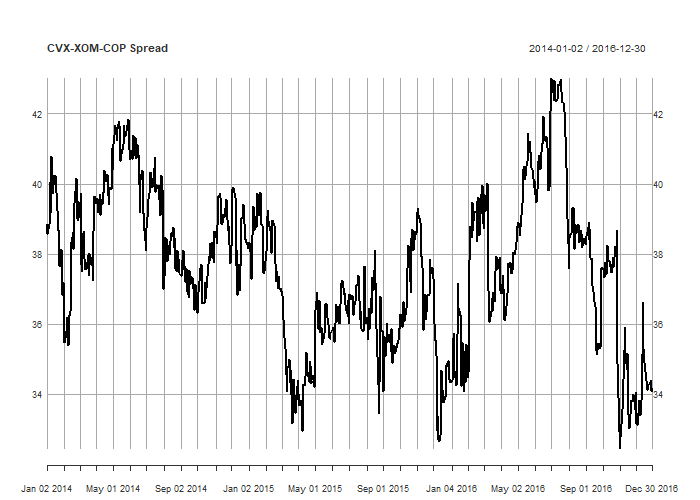
For completeness, here’s an example of using the Johansen test on a portfolio of three instruments, adding Conoco-Philips (COP, another energy company) to our existing pair:

# 3-series johansen example

portfolio <- load_data(c('XOM', 'CVX', 'COP'), start='2014-01-01', end='2017-01-01', source='yahoo', 
                       return_data = 'Adjusted', save_indiv = TRUE)

plot(portfolio, col=c('blue', 'red', 'black'), main = 'XOM and CVX')
legend('bottomright', col=c('blue', 'red', 'black'), 
       legend=c('XOM', 'CVX', 'COP'), lty=1, bty='n')

jt <- ca.jo(portfolio, type="eigen", K=2, ecdet="const", spec="longrun")
summary(jt)

'''
output:
###################### 
# Johansen-Procedure # 
###################### 

Test type: maximal eigenvalue statistic (lambda max) , without linear trend and constant in cointegration 

Eigenvalues (lambda):
  [1]  1.696099e-02  6.538698e-03  2.249865e-03 -3.753129e-18

Values of teststatistic and critical values of test:
  
          test 10pct  5pct  1pct
r <= 2 |  1.70  7.52  9.24 12.97
r <= 1 |  4.95 13.75 15.67 20.20
r = 0  | 12.90 19.77 22.00 26.81
 
Eigenvectors, normalised to first column:
  (These are the cointegration relations)

XOM.Adjusted.l2 COP.Adjusted.l2 CVX.Adjusted.l2   constant
XOM.Adjusted.l2      1.00000000       1.0000000        1.000000  1.0000000
COP.Adjusted.l2      0.05672729      -0.5610875        1.169714  0.3599442
CVX.Adjusted.l2     -0.49143408      -0.7078675       -1.764155 -1.2310314
constant           -37.60449105      19.0946477       31.146100  9.2824197

Weights W:
  (This is the loading matrix)

XOM.Adjusted.l2 COP.Adjusted.l2 CVX.Adjusted.l2      constant
XOM.Adjusted.d     -0.04560861     0.003903014    -0.001297751 -1.251443e-15
COP.Adjusted.d     -0.01296028     0.003347451    -0.003035065 -5.016783e-16
CVX.Adjusted.d     -0.02437064     0.009714253    -0.001897541 -5.504833e-16
'''

# Johansen spread
jo_hedge <- jt@V[, 1]
jo_spread <- portfolio%*%jo_hedge[1:3]
jo_spread <- xts(jo_spread, order.by = index(portfolio))
plot(jo_spread, main='CVX-XOM-COP Spread', col='black')

Take care!

While it may seem tempting to check thousands of instrument combinations for cointegrating relationships, be aware of these two significant issues:

1. Doing this indiscriminately will incur significant amounts of data mining bias. Remember that if you run 100 statistical significance tests, 5 will pass at the 95% confidence level through chance alone.
2. The Johansen test creates portfolios using all components. This can result in significant transaction costs, as for every instrument added, further brokerage and spread crossing costs are incurred. One alternative is to explore the use of sparse portfolios – see for example this paper.

Practical advice

In practice, I use statistical tests such as CADF and Johansen to help find potential hedge ratios for price series that I think have a good chance of generating a profit in a pairs trading strategy. Specifically, I don’t pay a great deal of attention to the statistical significance of the results. The markets are noisy, chaotic and dynamic, and something as precise as a test for statistical signficance proves to be a subotpimal basis for making trading decisions.

In practice, I’ve seen this play out over and over again, when spreads that failed a test of statistical signifiance generated positive returns out of sample, while spreads that passed with flying colours lost money hand over fist. Intuitively this makes a lot of sense – if trading was as easy as running tests for statistical significance, anyone with undergraduate-level math (or the ability to copy and paste code from the internet) would be raking money from the markets. Clearly, other skills and insights are needed.

In future posts, I’ll show you some backtesting tools for running experiments on pairs trading. Thanks for reading!

 

Looking for a simpler, effective approach?

We just launched our new FX Bootcamp, where you can team up, build and trade a live retail algo FX portfolio from scratch in just 16 weeks. Not only will you end up with a diverse, robust portfolio by the end, but you will have gained the exact approach we’ve used to trade for a living for decades between us.

Interested?

Enrolment to FX Bootcamp will close Midnight Friday July 12th. Join your new team of retail traders and get started!