Parameter Optimisation for Systematic Trading

Optimisation tools have a knack for seducing systematic traders.

And what’s not to love?

Find me the unique set of parameters that delivered the greatest return in my ten-year backtest. And do it in under five seconds.

That’s certainly attractive.

But do you want to hear something controversial?

When it comes to the parameters of a systematic trading strategy, in the majority of cases optimisation is your enemy. A siren, luring you to shipwreck.

On the other hand, there are a few applications of optimisation that are helpful and sensible in a trading context. Usually however, they’re not obvious.

So we decided to write a series of blog posts to give you the no-holds-barred low-down on optimisation for systematic trading. We’ll start with a lightning tour of various optimisation techniques (this article) before moving on to:

• The implicit assumptions you make when you optimise strategy parameters
• Best practices related to optimisation of strategy parameters
• Optimisation use cases in the context of systematic trading

Optimisation tools and techniques

Let’s start with a whirlwind tour of a selection of optimisation tools. We’ll explore these by way of the Zorro trading platform, which has a number of powerful optimisation algorithms built in.

Setting up for optimisation

To make Zorro optimise a strategy’s parameters, you need to set the PARAMETERS flag and assign calls to the optimize function to the parameters you wish to tune.

Here’s what this looks like for a simple long-only moving average system where we optimise the length of the moving average window:

function run()  
{  
    LookBack = 200;  // cover the largest possible lookback from the optimize call below
        set(PARAMETERS);  
    
    // strategy parameters
    var window_length = optimize(100, 20, 200, 20);  // optimise moving average window length
    vars closes = series(priceClose());  // a time series of closing prices
    vars ma = series(SMA(closes, window_length));  // a time series of moving average of closing prices
    
    // trade logic
    if(crossOver(closes, ma))
    {
        enterLong();
    }
    else if(crossUnder(closes, ma))
    {
        exitLong();
    }
}

The optimize call in line 7 gets four numbers as arguments:

• The first (100) is the default window length value
• The second (20) and third (200) define the range of values to optimize over
• The fourth (20) defines the step size

So in this example, Zorro would test the values 20, 40, 60, 80, … etc all the way up to 200.

It would store the “best” value in a text file, and then use that value whenever you run this script with the PARAMETERS flag set.

How does Zorro define the “best” value?

That’s a great question.

Whenever a parameter is optimised, it needs to be optimised towards a specific goal. The best value could be the one that maximised return, minimised drawdown, maximised Sharpe ratio, or something else entirely.

Each of these goals would likely have a different optimal parameter value.

By default, Zorro uses the Pessimistic Return Ratio (PRR) as its goal (referred to as an objective function). PRR is a profit factor (ratio of gross wins to gross losses) penalised for lower numbers of trades and with the impact of outlying wins and losses dampened.

We might be more interested in maximising risk adjusted returns, in which case we could implement an objective function based on the Sharpe ratio. That’s simply a matter of writing a custom function named objective that returns the quantity you want maximised, and including it in your script.

Here’s what that looks like for our n-day moving average strategy:

// sharpe ratio objective function
var objective()
{
  if(!NumWinTotal && !NumLossTotal) return 0.;
  return ReturnMean/ReturnStdDev;
}


function run()  
{  
    LookBack = 200;  // cover the largest possible lookback from the optimize call below
    set(PARAMETERS);  
    
    // strategy parameters
    var window_length = optimize(100, 20, 200, 20);  // optimise moving average window length
    vars closes = series(priceClose());  // a time series of closing prices
    vars ma = series(SMA(closes, window_length));  // a time series of moving average of closing prices
    
    // trade logic
    if(crossOver(closes, ma))
    {
        enterLong();
    }
    else if(crossUnder(closes, ma))
    {
        exitLong();
    }
}  

Zorro has access to a number of trade- and strategy-level statistics.

Here, we use NumWinTotal and NumLossTotal (the number of winning and losing positions respectively) to return zero if the strategy didn’t enter any positions.

ReturnMean and ReturnStdDev are the mean and standard deviation of return on investment on a bar-by-bar basis. That is, if your strategy was based on daily price bars, then ReturnMean and ReturnStdDev would be based on daily strategy returns.

Some other interesting strategy-level statistics that Zorro makes available include DrawDownMax , DrawDownBars and ReturnR2 (the similarity of the strategy’s equity curve with a straight line).

Is maximising an objective function the smartest approach?

Here’s a plot of a hypothetical strategy’s performance as a function of the value chosen for one of its parameters:

If your goal was maximising Sharpe ratio, you’d choose a value of 170. But does that seem like a sensible choice?

Of course, you intuitively get the sense that the outperformance of that value is a little shaky. The values immediately around it don’t do nearly as well, which implies that the market wouldn’t need to look all that different in the future for this thing to fall over badly. And of course the market is going to look different in the future.

On the other hand, the lower but more stable region of performance in the left of the plot implies a degree of robustness. The strategy is rather insensitive to changes in this region. That bodes well for future performance.

This illustrates a key point:

In strategy development, our goal is not to maximise backtest performance; it’s to optimise for future robustness.

Picking outlying points on the parameter space is not optimising for future robustness.

Picking regions of parameter stability can help (although it’s rarely enough – a point to which we’ll return later).

By default, Zorro optimises towards plateaus like we see in the left of the plot. In this case, it would pick a value around 60.

If for some reason we wanted Zorro to pick the highest single peak, we need to set a TrainMode flag like this:

setf(TrainMode, PEAK);

Next, let’s explore some different approaches to parameter optimisation.

Ascent optimisation

In this approach (Zorro’s default), we optimise each parameter independently. For a strategy with three parameters to optimise, it works like this:

1. Optimise the first parameter while holding the other parameters constant at their default values.
2. Optimise the second parameter holding the first parameter at its optimised value and the third value to its default.
3. Optimise the third parameter holding the first and second parameters at their optimised values.

Ascent optimisation is fast and reduces the scope for overfitting at the cost of not fully exploring the parameter space. The order in which parameters appear in the script matters.

Brute force optimisation

This is the kitchen sink approach where we try every possible combination of parameter values and pick the one we like best.

To put Zorro into brute force mode, simply add the line setf(TrainMode, BRUTE) to the script.

In brute force mode, Zorro won’t use the step parameter of the optimize function. Instead, it will divide the range into ten equal steps. You can omit this parameter in brute force mode, but if you supply it, Zorro will ignore it.

Genetic optimisation

Genetic optimisation is a heuristic approach based on evolutionary principles. A population of parameter combinations are iteratively selected, recombined and mutated randomly to form successive generations, with the best offspring surviving into the next iteration.

Zorro’s genetic optimisation routine considers every possible parameter combination an individual in the original population, but then evolves those individuals towards an optimal solution.

It can be configured by setting the parameters Population (the number of fittest individuals to retain in each generation), Generations (the maximum number of iterations), and MutationRate (the average number of random mutations in each generation). However, the default settings are normally fine to start with.

Genetic optimisation can be a useful technique when it isn’t feasible to try every combination of values, or when parameters affect one another in non-linear or complex ways. However, it will normally overfit drastically to financial data due to the inherently low signal to noise ratio.

Splitting data for optimisation

It’s good practice to test optimised parameters on unseen or out-of-sample data. Zorro provides a number of ways to do this out of the box.

Horizontal split

This method creates a single training set and a single test set, but splits them up such that by default every third week is set aside for testing:

To set it up, skip the relevant weeks using the SKIP flags:

function run() 
{
  if(Train) set(PARAMETERS+SKIP3);
  if(Test) set(PARAMETERS+SKIP1+SKIP2);
  ...
}

You can change the default number of bars skipped using Zorro’s DataSkip parameter.

This method is fast and makes reasonably good use of the available data.

Vertical split

In this approach, the training and testing sets are continuous and adjacent to one another:

Define the amount of data in the training and testing sets using the DataSplit parameter:

function run() // vertical split optimization
{
  set(PARAMETERS);
  DataSplit = 75; // 75% training, 25% test period
  ...
}

Again, this approach is fast and makes a reasonable use of the available data.

Walk-forward

This method splits data into training and testing sets on a rolling basis:

It takes a little longer than the other approaches but more accurately reflects the trading of a strategy that was re-optimised periodically.

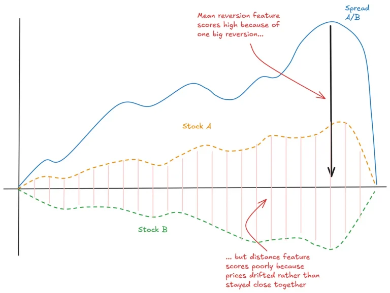
An example

Here’s an example of walk-forward optimising a pairs trade on two energy companies, Conoco Philips and Exxon Mobil.

The strategy constructs a spread from the price series of the two stocks and a hedge ratio. It then calculates a z-score of that spread and goes long or short the spread as the z-score crosses various levels. We have a maximum of six potential entries at a time.

The parameters to be optimised are:

• hedge ratio
• z-score lookback
• spacing between levels

We split our training-testing data 80-20 by setting DataSplit = 80 and we use 300 days total in each walk-forward cycle by setting WFOPeriod = 300.

Here’s the code:

/* Z-SCORE PAIRS TRADING

*/

#define Asset1 "CVX"
#define Asset2 "XOM"
#define MaxTrades 6

int Portfolio_Units = 10; //units of the portfolio to buy/sell (more --> better fidelity to dictates of hedge ratio)

var calculate_spread(var hedge_ratio)
{
  var spread = 0;
  asset(Asset1); spread += priceClose();
  asset(Asset2); spread -= hedge_ratio*priceClose();
  return spread;
}

function run()
{
    set(PARAMETERS, PLOTNOW, TESTNOW);
    setf(TrainMode, GENETIC);
    StartDate = 2010;
    EndDate = 2020;
    BarPeriod = 1440;
    LookBack = 200;
    MaxLong = MaxShort = MaxTrades;
    assetList("AssetsSP50");
    DataSplit = 80;
    WFOPeriod = 350;
    
    if(is(INITRUN)) 
    {
        asset(Asset1);
        assetHistory(Asset, FROM_AV);
        asset(Asset2);
        assetHistory(Asset, FROM_AV);
    }
    
    // optimisation parameters
    var beta = optimize(1, 0.2, 5, 0.2);
    var zscore_lookback = optimize(100, 20, 100, 20);
    var level_spacing = optimize(1, 0.1, 0.5, 0.1);  // number of zscores between trade entries
    
    vars spread = series(calculate_spread(beta));
    vars ZScore = series(zscore(spread[0], zscore_lookback));
    
    // set up trade levels
    var Levels[MaxTrades]; 
    int i;
    for(i=0; i<MaxTrades; i++)
    {
        Levels[i] = (i+1)*level_spacing;
    }
    
    // trade logic
    if(crossOver(ZScore, 0)) exitLong("*");
    if(crossUnder(ZScore, 0)) exitShort("*");
    
    for(i=0; i<MaxTrades; i++)
    {
        if(crossUnder(ZScore, -Levels[i])) 
        {
            asset(Asset1);
            Lots = Portfolio_Units;
            enterLong();
            asset(Asset2);
            Lots = Portfolio_Units * beta;
            enterShort();
        }
        if(crossOver(ZScore, Levels[i])) 
        {
            asset(Asset1);
            Lots = Portfolio_Units;
            enterShort();
            asset(Asset2);
            Lots = Portfolio_Units * beta;
            enterLong();
        }
    }
    
    for(i=1; i<MaxTrades-1; i++)
    {
        if(crossOver(ZScore, -Levels[i])) 
        {
            asset(Asset1);
            exitLong(0, 0, Portfolio_Units);
            asset(Asset2);
            exitShort(0, 0, Portfolio_Units * beta);
        }
        if(crossUnder(ZScore, Levels[1])) 
        {
            asset(Asset1);
            exitShort(0, 0, Portfolio_Units);
            asset(Asset2);
            exitLong(0, 0, Portfolio_Units * beta);
        }
    }

    // plots
    plot("zscore", ZScore, NEW, BLUE);
    int i;
    for(i=0; i<MaxTrades; i++)
    {
        plot(strf("#level_%d", i), Levels[i], 0, BLACK);
        plot(strf("#neglevel_%d", i), -Levels[i], 0, BLACK);
    }   
    plot("spread", spread, NEW, BLUE);
}

This is just a toy example – not a trading script.

And here’s a short recording of Zorro blasting through the ascent-based walk-forward optimisation and simulation. Following that, you’ll see a demonstration of the same walk-forward but using the genetic optimiser.

The reality

Did you notice in the video that the walk-forward that used the genetic optimiser did much worse?

Sure, this is just a single example, but that’s not an unusual result.

Genetic optimisation is a powerful tool – it will zero in on anything that helps drive the objective function toward its goal, regardless of whether it’s a real effect or just noise.

The ascent optimisation approach doesn’t solve this either. At least, not in the sense of distinguishing between real effects and noise.

Really, it’s attempting to save the user from him or herself by reducing the search space and hence the scope for overfitting. Which is a useful thing, but doesn’t get to the heart of the issue.

The only way to distinguish between real effects and noise is to do deep, detailed research in an effort to understand the effect as best you can. This means gathering evidence that shines light on questions such as:

• What do I think is the driver of the effect? Where’s the risk premium or limit to arbitrage?
• How consistent is the effect over time?
• Is it robust to any simple way of capturing it?
• Is it present if I look broadly across other assets?

This requires some hard work, clear thinking and the ability to not give yourself a free pass.

Using an optimiser early in the research process essentially skips these important steps. It hides the detail, limits your understanding, and short-circuits your opportunity to add to your knowledge of the market.

Think about it like this. If strategy development were as simple as clicking an optimise button on some software, then every geek with a modern laptop would be killing it in the markets. Clearly that’s not the case. There’s more to strategy development – much more.

Conclusions and next steps

In this post we’ve explored parameter optimisation in Zorro. In particular, you’ve seen how Zorro makes it incredibly easy to use a variety of optimisation tools and data splitting approaches.

I also hit you with something of a reality check in which I essentially told you to avoid parameter optimisation.

I hope that didn’t take the wind out of your sails too much. Instead, I hope that the thought of taking a deep dive into your trading ideas in an effort to understand them on a new level excites you. The best traders I’ve ever met all share this excitement – they tend to approach the market like curious scientists hunting for deep understanding, rather than being content to accept the output of an optimisation algorithm.

Having said all that, there are use cases for optimisation in systematic trading.

In the next post, we’ll explore these use cases in more detail and I’ll also tell you my best practices for optimisation in systematic trading.