Exploring mean reversion and cointegration with Zorro and R: part 1

This series of posts is inspired by several chapters from Ernie Chan’s highly recommended book Algorithmic Trading. The book follows Ernie’s first contribution, Quantitative Trading, and focuses on testing and implementing a number of strategies that exploit measurable market inefficiencies. I’m a big fan of Ernie’s work and have used his material as inspiration for a great deal of my own research. My earlier posts about accounting for randomness (here and here) were inspired by the first chapter of Algorithmic Trading. Ernie works in MATLAB, but I’ll be using R and Zorro.
Ernie cites Daniel Kahneman’s interesting example of mean reversion in the world around us: the Sports Illustrated jinx, namely that “an athlete whose picture appears on the cover of the magazine is doomed to perform poorly the following season” (Kahneman, 2011). Performance can be thought of as being randomly distributed around a mean, so exceptionally good performance one year (resulting in the appearance on the cover of Sports Illustrated) is likely to be followed by performances that are closer to the average.
Mean reversion also exists in, or can be constructed from, financial time series data. In this context, I will refer to data that tends to mean revert as stationary. Note that stationarity does not imply a range-bound price series with variance independent of time, rather that the variance simply increases more slowly than that of a normal diffusion process (yes, I know there are more formal and robust definitions of stationarity, but since we are only interested in the practical application of the concept to trading, this will do for now and you can stop cringing).  In this post, I’ll explore mean reversion of individual time series and in the next post will investigate constructing artificial mean reverting time series. Of course, I’ll propose trading strategies based on the findings.

Augmented Dickey-Fuller Test

If the time series is not a random walk, the current value tells us something about the next value in the series. If the series is mean reverting, a value above the mean will more likely be followed by a down move and vice versa. The Augmented Dickey-Fuller (ADF) test is a test for the tendency of the series to mean revert based on this observation.
Using a linear model of price changes:

Δy(t) = λy(t − 1) +βt + μ + α1Δy(t − 1) + … + αkΔy(t − k) + εt

where Δy(t) ≡ y(t) − y(t − 1),  Δy(t − 1) ≡ y(t − 1) − y(t − 2), etc.

we can see that if λ ≠ 0, then Δy(t) depends on the current level y(t − 1) and therefore is not a random walk. The ADF test examines whether the hypothesis λ = 0 can be rejected at a given confidence level.
The following R code (truncated here, full code linked below) examines mean reversion of daily price data for the AUD/NZD exchange rate for the period 2008 to mid-2015. The code uses the ur.df  function from the urca  package, which contains a number of econometric functions. There is also the adf.test  function from the tseries  package, but this implementation includes only one of the three variations of the ADF test, and the particular implementation in that package is not suitable for this case. In this application, we should set the drift term to zero because the constant drift in price tends to be of a much smaller magnitude than the daily fluctuations in price (Chan, 2013).  The intercept however should be non-zero. This combination is achieved by using the drift  argument of the ur.df  function. In addition, Chan suggests starting with a lag of 0, but that better results are usually obtained with a lag of 1, which may indicate serial correlation of price changes.

library(zoo)
library(urca)
##########
#Import data
...
...
##########
# ADF test
summary(ur.df(audnzd, type = "drift", lags = 1))

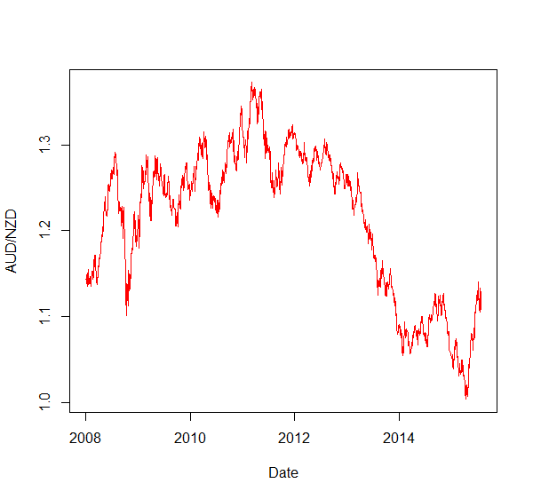
We may expect a degree of mean reversion in this time series given that each currency in the pair is a so-called commodity currency and the two countries inhabit the same corner of the globe. Therefore, they may share a number of market factors. However, the time series doesn’t look overly stationary:

The results of the ADF test are as follows:

###############################################
# Augmented Dickey-Fuller Test Unit Root Test #
###############################################
Test regression drift
Call:
lm(formula = z.diff ~ z.lag.1 + 1 + z.diff.lag)
Residuals:
      Min        1Q    Median        3Q       Max
-0.026807 -0.003564 -0.000072  0.003334  0.035011
Coefficients:
              Estimate Std. Error t value Pr(>|t|)
(Intercept)  0.0026755  0.0019258   1.389    0.165
z.lag.1     -0.0022207  0.0015837  -1.402    0.161
z.diff.lag  -0.0009535  0.0226825  -0.042    0.966
Residual standard error: 0.006004 on 1945 degrees of freedom
Multiple R-squared:  0.001015,	Adjusted R-squared:  -1.27e-05
F-statistic: 0.9876 on 2 and 1945 DF,  p-value: 0.3726
Value of test-statistic is: -1.4023 0.9922
Critical values for test statistics:
      1pct  5pct 10pct
tau2 -3.43 -2.86 -2.57
phi1  6.43  4.59  3.78

In the urca  implementation, the λ term in our linear model above is the estimate of  z.lag.1 divided by its standard error, and our critical values corresponds to tau2. In this case, the test statistic is -1.402. This is greater than the the 10% critical value, so we can’t reject the null hypothesis that λ=0 with even 90% certainty and should conclude that the time series is therefore not mean reverting. Interestingly, the negative value for lambda indicates that the time series is at least not trending.

Hurst exponent

Another way of looking at stationarity and mean reversion is from the perspective of the speed of diffusion from an initial state. A stationary series would diffuse at a slower rate than a geometric random walk. We can measure the speed of diffusion as the variance of the series:

Var(τ) = 〈|z(t + τ) − z(t)|^2〉

where

• z = log(price)
• τ is an arbitrary time lag
• 〈…〉 is an average over all t’s

For a geometric random walk:

〈|z(t + τ) − z(t)|^2〉 ∼ τ

But if the series is either mean reverting or trending, this relationship will  not hold, and instead we get

〈|z(t + τ) − z(t)|^2〉 ∼ τ^2H

Where H is the Hurst exponent, H serves as an indicator of the degree to which a series trends. For a trending series, H > 0.5, for a mean-reverting series, H < 0.5 and for a geometric random walk, H = 0.5 (Chan, 2013).

The pracma package in R can be used to to calculate the Hurst exponent. See this for an interesting account of the origins of the Hurst exponent as well as a description of the pracma  implementation.

library(pracma)
# Hurst exponent
hurst <- hurstexp(log(audnzd)) # returns a list of various Hurst calculations

The hurstexp  function returns a list of variously corrected and modified values for H, whose determination is a problem of estimation more than a problem of calculation.

Simple R/S Hurst estimation: 0.8821693
Corrected R over S Hurst exponent: 1.00354
Empirical Hurst exponent: 0.9588154
Corrected empirical Hurst exponent: 0.9422138
Theoretical Hurst exponent: 0.5349181

These results suggest that the time series is not mean-reverting, but instead has a tendency to trend.

Half life of mean reversion

At this point, we can step away from the constraints of statistical tests and the demands of 95% confidence limits. One of the interesting aspects of trading is that it is sometimes possible to be profitable despite not achieving the demanding requirements of significance imposed by a statistical test. The challenge is understanding when such a situation may arise and when moving away from statistical significance is likely to lead to disaster. One example of the former case may involve using a time series’ half life of mean reversion as the basis of a mean reversion strategy.
An alternate interpretation of the lambda coefficient defined above is the  time that a series takes to mean revert (Chan, 2013). To see this interpretation, simply transform the discrete time series model described above to a differential form. Ignoring the drift and lagged difference terms, the differential form is equivalent to the Ornstein-Uhlenbeck stochastic process.

dy(t) = (λy(t − 1) + μ)dt + dε

where ε is Guassian noise. This differential form leads to an analytical solution for the expected value of y(t):

E( y(t)) = y₀exp(λt) − μ/λ(1 − exp(λt))

which, for a mean reverting process with negative λ, tells us that the expected value of the price decays exponentially at a half-life of -log(2)/λ

If we determine λ to be positive, we can infer that the price series is trending and therefore should not be traded in a mean-reverting strategy. If λ is close to zero, the half life will be very long and any mean reverting strategy will necessarily require long holding times. If λ is very negative, it is more likely that a profitable and practical mean reversion strategy exists since the price series tends to revert to the mean quickly. In his discussion of this idea, Chan (2013) also asserts that λ should be used in calculating lookback periods of moving averages and standard deviations for a mean reverting strategy, with a small multiple of λ often being optimal.

The following R code calculates the half life of mean reversion of our AUD/NZD exchange rate data. To determine λ, regress y(t) − y(t − 1) against y(t − 1):

##########
# Calculate half life of mean reversion
y <- audnzd
y.lag <- lag(y, -1)
delta.y <- diff(y)
df <- cbind(y, y.lag, delta.y)
df <- df[-1 ,] #remove first row with NAs
regress.results <- lm(delta.y ~ y.lag, data = df)
lambda <- summary(regress.results)$coefficients[2]
half.life <- -log(2)/lambda

In this case, the half life is calculated to be 311 days. At first glance, this feels far too long for this impatient trader! Below I will present a simple trading strategy to test whether this series is exploitable via mean reversion methods.

A simple linear mean reverting strategy

A simple linear mean reverting strategy is realised by determining the normalised deviation of price from its moving average (essentially, a moving Z-score of the last closing price) and holding a position negatively proportional to this deviation. The lookback period for the moving average and moving standard deviation is set equal to the half life of mean reversion. Of course, a moving average and moving standard deviation are required because even though we implicitly assume a stationary price series, in reality it is likely to evolve. In addition, the variance of a mean reverting process does change with time, albeit not as quickly as a geometric random walk.
The Zorro code below implements this linear strategy. The number of lots held is equivalent to the negative of the Z-score to account for the fact that a positive Z-score implies a downwards reversion and a negative Z-score implies a positive reversion. Note that the market value is units of the quote currency (AUD in this case). If this is not the account currency, an allowance would need to be made for converting the profits and losses to the account currency.
The presentation of this strategy is intended as a proof of concept only and is not practical for live trading. Transaction costs are excluded from the analysis, but would likely be significant given the constant rebalancing of the position. There is also some look ahead bias in that the lookback period for the Z-score calculations was derived from the price history being traded. In the next post, I’ll introduce some examples of more practical methods for exploiting mean reversion.

int lotsOpen() {
	string CurrentAsset = Asset;
	int val = 0;
	for(open_trades)
	if(strstr(Asset,CurrentAsset) && TradeIsOpen)
	val += TradeLots;
	return val;
}
function run() {
	set(LOGFILE);
	BarPeriod = 1440;
	StartDate = 2008;
	EndDate = 2015;
	Spread =	Slippage = RollShort = RollLong = 0; // set transaction costs to zero
	PlotWidth = 750;
	int halfLife = 311;
	LookBack = halfLife+1;
	vars Close = series(priceClose());
	vars zScore = series(10*(-(Close[0] - SMA(Close, halfLife))/StdDev(Close, halfLife))); // multiply by 10 as minimum lot size is 1
	int openLots;
	if (zScore[0] > 0) { //want to be long the asset
		exitShort();
		openLots = lotsOpen();
		if (openLots < zScore[0]) {//need to buy more
			Lots = zScore[0] - openLots;
			enterLong();
		}
		else if (openLots > zScore[0]) {
			exitLong(0,0,(openLots - zScore[0])); //need to close some
		}
	}
	else if (zScore[0] < 0) { //want to be short the asset
		exitLong();
		openLots = lotsOpen();
		if (openLots < abs(zScore[0])) { //need to sell more
			Lots = abs(zScore[0]) - openLots;
			enterShort();
		}
		else if (openLots > abs(zScore[0])) {
			exitShort(0,0,(openLots - abs(zScore[0])));
		}
	}
	plot("zScore", zScore, NEW, BLUE);
	plot("MAve", SMA(Close, halfLife), NEW, GREEN);
	plot("MSD", StdDev(Close, halfLife), NEW, RED);
}

The strategy returns a respectable 22% per annum, albeit with a significant drawdown and a Sharpe ratio of only 0.39:

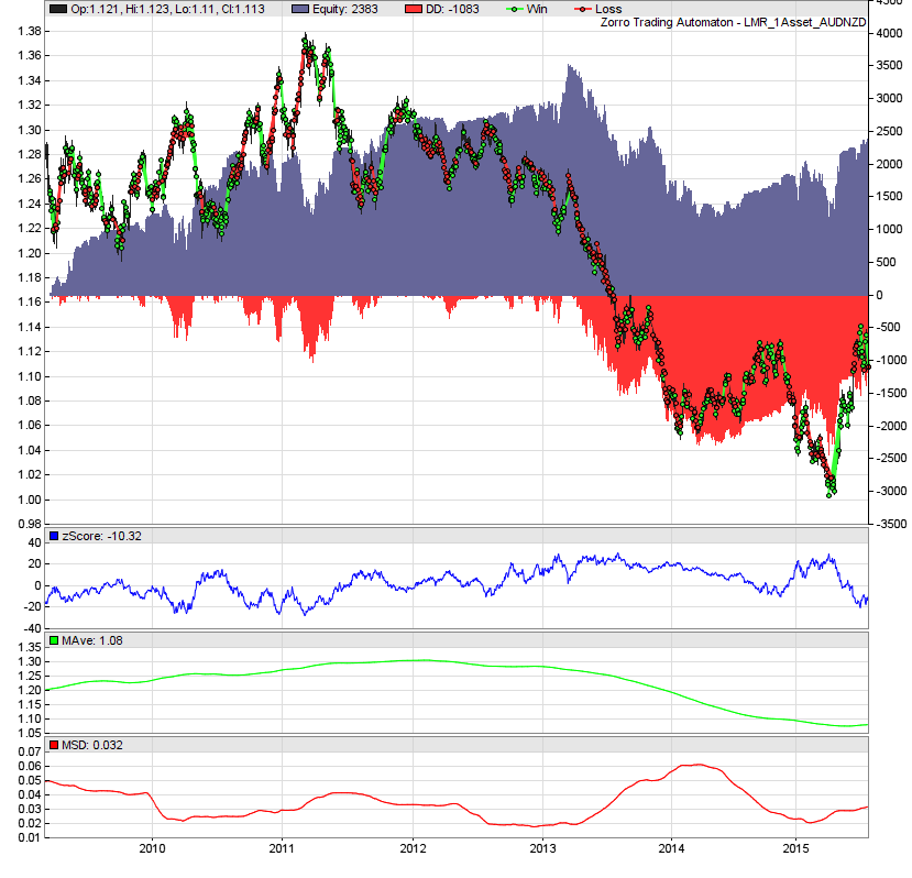
Interestingly, note how the strategy suffers its greatest drawdown at the same time as price breaks its multi-year low in early 2013 and then trends strongly to what appears to be a new range. Note the behaviour of the moving average and the moving standard deviation during this period: their rates of change both increase dramatically. This implies a simple filter based on the rate of change of these series, which leads predictably to a tempering of the maximum drawdown:

// simple filter based on rate of change of moving average
vars ma = series(SMA(Close, halfLife));
vars delta = series(100 *(ma[0] - ma[1]));
var threshold = 0.045;
if (abs(delta[0]) < threshold) {
...
// trade normally //
...
}
else if (abs(delta[0]) > threshold) { // exit open trades if rate of change exceeds threshold
	exitLong("*"); exitShort("*");
}
plot("delta", delta, NEW, BLUE);

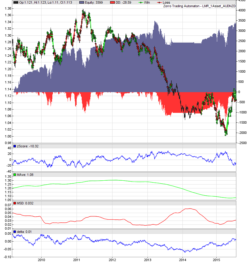
The threshold  parameter, which controls the operation of the filter, is an optimization parameter that may or may not hold up out of sample. There are of course numerous options for detecting so-called ‘regime change’ – in this context, when a price series transitions from having a mean-reverting character to trending – including, for example, a rolling ADF test, the Hurst exponent, even the half life of mean reversion itself, or more generally, the coefficient obtained by regressing the bar-to-bar price change against the lagged price. These, and the many other examples, each have their own pros and cons. Personally, I prefer a filter based on the actual performance of the strategy and which starts and stops the algorithm upon the crossing of the theoretical equity curve with a filtered version of itself (credit to the Zorro team for introducing me to that idea). This approach has the happy side effect of preventing catastrophic losses if the price series being traded fundamentally changes and ceases to mean revert, or at least does so for long enough to wipe out a trading account. This is a very real prospect; it is trivial to see that many price series exhibit varying periods of predominantly trending or mean reverting behaviour, however predicting the change point and using that knowledge in a practical trading strategy is certainly non-trivial. To me, it makes sense to respond to something we can know with certainty (the current performance of the strategy in real time), particularly when that knowledge is a good indicator of the breakdown of the fundamental assumptions underlying the strategy.
I have also found that, in general, reducing the lookback period of the moving average and standard deviation used in the Z-score calculation to approximately half the calculated half life of mean reversion improves performance. Reducing the lookback period further tends to result in deteriorating performance. Below is the performance for a lookback of 150, as opposed to the calculated half life of mean reversion of 311, with no rate of change filter:

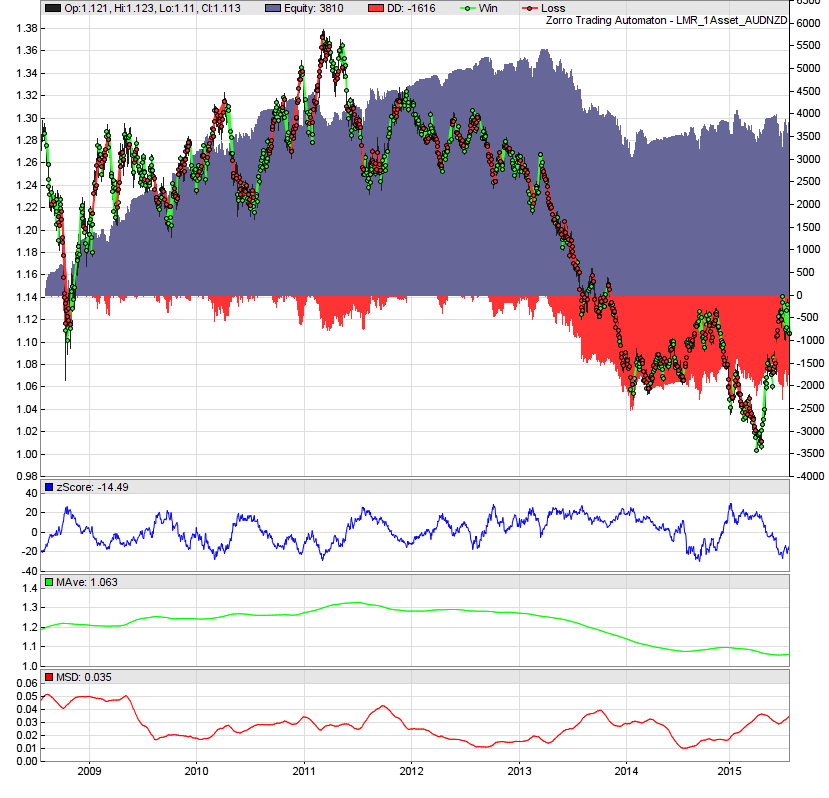
The annual return is 32% and the Sharpe ratio is 0.48. If I include transaction costs of 1.7 points per side and simulate slippage by delaying orders by ten seconds, the annual return is 25% and the Sharpe ratio is  0.4.

Why use statistical tests?

Chan (2013) poses the question as to why bother with statistical tests for stationarity at all when, as traders, our overriding goal is to simply determine whether a given mean reversion strategy’s performance is good enough to invest money in. Couldn’t we just run a backtest and infer all the information we need? It turns out that the statistical significance of these stationarity tests is usually far higher than that obtained through a simple backtest. The reason is that such tests make use of the data embodied in every single sample (that is, bar) of the price series. In comparison, a backtest has only the number of completed trades, which is usually far less (the linear strategy presented here is something of an exception, although it is not really a strategy that anyone intends to trade as is). In addition, most strategies’ performance is dependent on a set of parameters that are largely external to the price series itself, further confusing the idea of statistical significance (this is one reason to prefer strategies with as few external parameters as possible). On the other hand, given a price series that passed the statistical tests for stationarity, or has a sufficiently short half life of mean reversion, we can be confident that a profitable mean reversion strategy exists – possibly just not the subject of our backtest.

Next steps

In the next part of this series, I’ll look into constructing artificial stationary time series and will present a more practical trading strategy for exploiting mean reversion.

Files used in this post

Here you can download a zip file containing the data and source code used in this post.
MeanReversionPart1

References

Chan, Ernest, 2013. Algorithmic trading, John Wiley and Sons, New Jersey
Kahneman, Daniel, 2011. Thinking, Fast and Slow, Farrar, Strauss and Giroux, New York