Back to Basics Part 3: Backtesting in Algorithmic Trading

This is the final post in our 3-part Back to Basics series. You may be interested in checking out the other posts in this series:

• Part 1: An Introduction to Algorithmic Trading
• Part 2: How to Succeed at Algorithmic Trading

We’ve also compiled this series into an eBook which you can download for free here.

Nearly all research in algorithmic trading is empirical. It’s based on observation and experience, unlike theory, which rests on assumptions, logic, and mathematics.

We often begin with a theoretical model, say, a time-series framework that we think describes the data, and then use empirical methods to test those assumptions. But no one would risk money on a model without first checking it against real observations. Every model is built on assumptions, and to my knowledge, no one has ever devised a complete model of markets from first principles.

Empirical research, then, is always central to developing trading systems. The challenge is that experiments often require thousands of observations. Market data arrives in real time, so collecting enough can take ages. Make a mistake in setup, or come up with a new idea, and you’re back to the beginning. It’s a painfully slow way to learn.

The alternative is simulation. By running experiments on historical data, we can compress time and test countless variations. In trading, this process is called backtesting. It gives immediate feedback on how an idea might have worked in the past. Of course, backtesting is hardly perfect, it comes with its own set of traps. That’s what this article sets out to explore.

Why Backtesting Matters in Algorithmic Trading?

Before I get too deep into backtesting theory and practice, I want to step back and ask why we’d backtest at all. I’ve already said it lets us do empirical research quickly and efficiently. But do we really need that? I mean, everyone knows you just buy when the RSI drops below 30, right?

Obviously, that was rhetorical. My point is to call out a subtle but dangerous way of thinking that sneaks in if we’re not careful. I know most Robot Wealth readers already get this, but over the last couple of years I’ve worked with plenty of people from non-mathematical or non-scientific backgrounds who struggle with it, sometimes without even realising. This feels like the right place to address it.

The Illusion of Simple Trading Rules

In a deterministic world, well-defined cause and effect, natural phenomena can be captured by neat mathematical equations. Engineers and scientists will think immediately of Newton’s laws: clear rules that predict outcomes from initial conditions, solvable with high school maths.

Markets, though, aren’t deterministic. The information we digest doesn’t map cleanly to future states. The RSI dropping below 30 doesn’t cause prices to rise. Sometimes prices rise, sometimes they fall, sometimes nothing happens at all. At best, we can say more buyers than sellers pushed things around.

Most people accept this. Yet I’ve seen the same people who admit markets aren’t deterministic follow trading rules simply because they read them in a book or online.

Why? I have a few theories, but the strongest is that it’s easy to believe what we want to believe. And nothing is more appealing than the idea that repeating a simple action will make you rich. It’s a seductive trap, even if your rational mind knows better and you haven’t questioned the assumptions behind that system you adopted.

I’m not suggesting all DIY traders fall for it, but I’ve noticed it often enough. If you’re new to trading, or struggling for consistency, it’s worth reflecting on.

Backtesting as a Reality Check

I hope it’s clear now why backtesting matters. Some trading rules will make money, most won’t. And the ones that do don’t work because they describe natural laws, they work because they capture some market trait that, over time, tilts the odds in your favour. You can never know how any single trade will turn out, but you can sometimes show that, in the long run, your chances look pretty good. Backtesting on past data gives us the framework to test those ideas and see whether the evidence supports them or not.

Simulation vs Reality in Backtesting

You might have noticed that in the descriptions of backtesting above I used the words simulation of reality and how our model might have performed in the past. These are very important points! No simulation of reality is ever exactly the same as reality itself. 

All Models Are Wrong, Some Are Useful

Statistician George Box said it best: “All models are wrong, but some are useful” (Box, 1976). The key is making our simulations useful, or fit for purpose. A monthly ETF rotation strategy doesn’t need the same detail as a high-frequency stat-arb model. What matters is that the simulation is accurate enough to support real decisions about allocating to a strategy.

So how do we build a backtesting environment we can trust as a decision-support tool? It’s not trivial. Biases and pitfalls lurk everywhere, and they can throw results completely off. But that’s part of the appeal. In my experience, the people drawn to algorithmic trading rarely shy away from a challenge.

Fit for Purpose, Not Perfect

At its simplest, backtesting means running your trading algorithm on historical data and tallying the profit and loss. Sounds straightforward, but in practice it’s alarmingly easy to produce inaccurate results or introduce bias that makes the whole exercise useless for decision-making.

To avoid that, we need to think about two things:

1. The accuracy of the simulation, and
2. The experimental framework we use to draw conclusions.

Both matter if you want any confidence in your results. I can’t stress enough how critical this is, get it wrong and all your effort is wasted. Most algorithmic traders pour countless hours into research and testing, and it’s tragic when poor methodology renders it meaningless. The next sections dig into these issues.

Ensuring Simulation Accuracy

If a simulation isn’t a close reflection of reality, what use is it? Backtests need to mimic real trading closely enough to serve their purpose. In theory, they should produce the same trades and results you’d get running the system live over the same period.

To judge accuracy, you need to understand how the backtest generates results, and where its limits lie. No model can perfectly capture the market, but a well-built one can still be useful if it’s fit for purpose. The goal is to get as close to reality as possible while staying conscious of the gaps. Even the best backtesting setups have them.

Backtesting accuracy can be influenced by:

Broker and Market Conditions

Trading conditions, spread, slippage, commission, swap, vary across brokers and setups, and they’re rarely static. The spread shifts constantly as orders enter and leave the book. Slippage, the gap between target and actual execution, depends on volatility, liquidity, order type, and execution latency. How you account for these moving parts can heavily influence simulation accuracy.

The right approach depends on the strategy. A high-frequency system pushed to capacity might require modelling the order book to capture liquidity. For a monthly ETF rotation strategy managing retirement savings, that level of detail would be unnecessary.

Data Granularity and Its Limits

The granularity of data, or sampling frequency, can make or break a simulation. Take hourly OHLC data: each bar provides only four points, so trades are evaluated once an hour. But what if both a stop loss and a take profit occur within the same bar? Without finer data, you cannot know which triggered first. Whether this matters depends on the strategy and how its entries and exits are defined.

Data Quality Issues

The accuracy of the data driving a simulation is critical. As the saying goes, “garbage in, garbage out.” Poor data leads to poor results. Market data is messy: outliers, bad ticks, missing records, misaligned time stamps, wrong time zones, duplicates. Stock data may need adjusting for splits and dividends. Survivorship bias can skew results by excluding bankrupt companies. OTC products like forex or CFDs may even trade at different prices depending on the broker, so one data set might not reflect another. How serious these issues are depends on the strategy and its use case.

The point is that many factors affect simulation accuracy, and they need to be understood in context so you can design the simulation sensibly. As with any scientific experiment, design is everything.

In practice, it helps to check accuracy before moving to production. One way is to run the strategy live on a small account, then simulate it on the same market data. Even with a good simulator, you will see small deviations. Ideally, they stay within a tolerance that does not change your allocation decision. If they do, your simulator probably is not accurate enough for the job.

Development Methodology and Common Biases

Beyond simulation accuracy, the experimental methodology itself can undermine results. Biases are often subtle but powerful, and they slip into research and development more easily than most people realise. Left unchecked, they can devastate live performance. That is why accounting for bias is critical at every stage of the process.

In Fundamentals of Algorithmic Trading, I outline a workflow to reduce these risks and a record-keeping method that helps spot bias in its many forms. Here, I will walk through the main biases that tend to creep in and how they affect a trading strategy. For a deeper dive, including the psychological traps that make bias so hard to avoid, see David Aronson’s Evidence-Based Technical Analysis (2006).

Understanding Look-Ahead Bias (Peeking Bias)

This bias appears when future knowledge influences trade decisions, using information that wasn’t available at the time. A simple example is taking an intraday trade based on the day’s closing price, which of course isn’t known until the session ends. Good simulators are designed to prevent this, but it is surprisingly easy to let it creep in when building your own tools.

When I use R or Python for modelling and testing, I often need to pay extra attention to this issue. The giveaway is usually obvious: an equity curve that looks unrealistically smooth, because predicting outcomes is easy when you already know the future.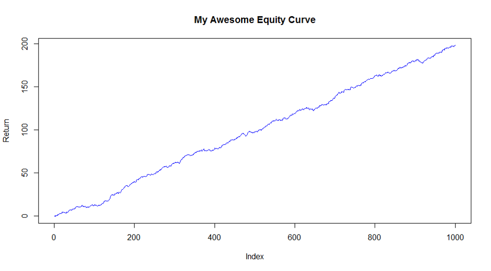

A subtler version occurs when parameters are calculated across the full simulation and then retroactively applied at the start of the next run. Portfolio optimisation settings are especially vulnerable to this form of look-ahead bias.

Understanding Curve-Fitting Bias (Over-Optimization)

This bias gives rise to “magical” backtests showing hundreds of percent annual returns. Needless to say, they’re useless in practice.

The plots below show curve-fitting at work. The blue dots are a simple linear function with noise added: y = mx + b + ϵ, where ϵ is random noise. We fit regression models of increasing complexity to the first 10 points (in-sample) and then tested them on the remaining 10 (out-of-sample). As model complexity increased, in-sample fit improved, but out-of-sample performance collapsed. The more complex the model, the worse the deterioration.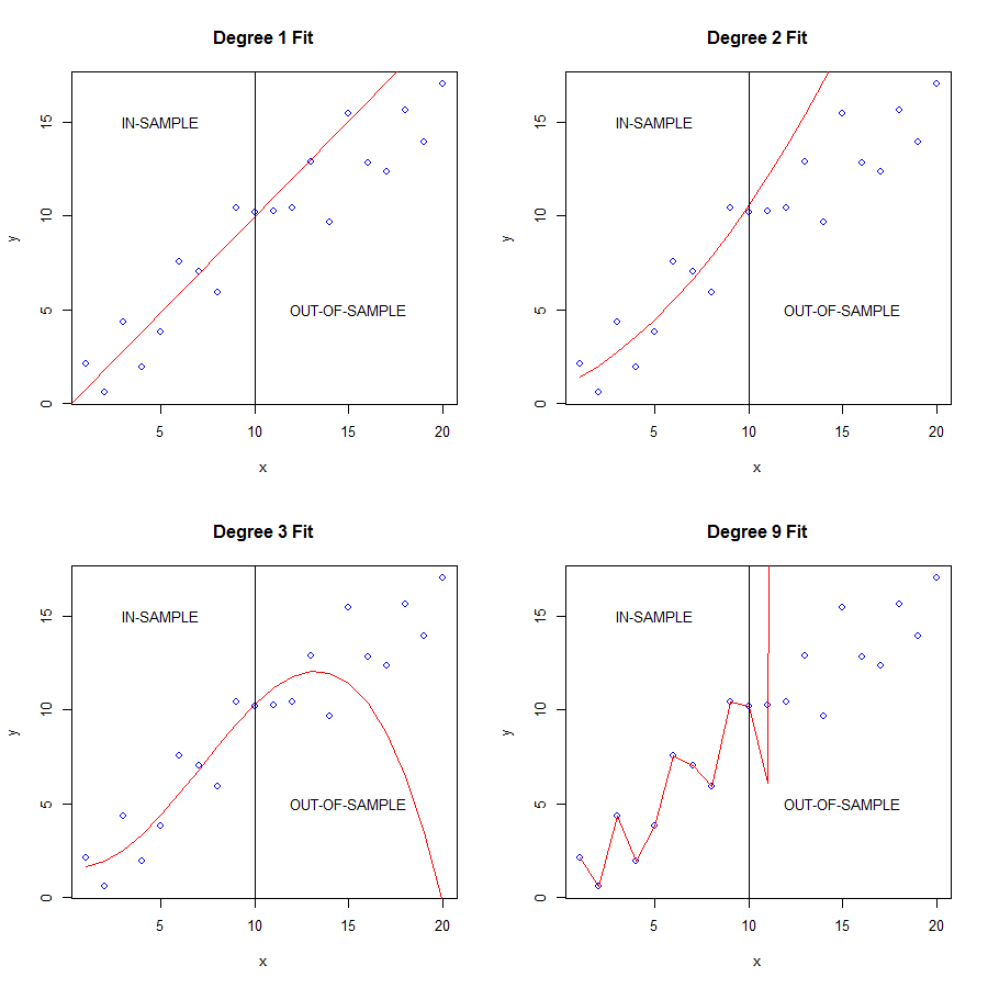

What’s happening is that complex models start fitting noise rather than signal. Since noise is random, predictions collapse once the model leaves the training set. Financial data is extremely noisy, so the danger is obvious: fit your strategy to the noise and you end up with a random trading model. That’s of little value to anyone, except your broker.

Understanding Data-Mining Bias (Selection Bias)

Data-mining bias is another major source of inflated model performance. It comes in many forms and is impossible to eliminate entirely, so the goal is to recognise it and account for it. The most common case is when you pick the best performer from a pool of algorithms, variants, variables, or markets. If you try enough combinations, you will eventually find one that looks good by chance.

For example, say you build a trend-following strategy for forex. It backtests well on EUR/USD but fails on USD/JPY. Choosing EUR/USD introduces selection bias, and your estimate of its performance on that pair is now upwardly skewed. The fix is to temper expectations or test it on new, unseen EUR/USD data for a more realistic performance estimate.

In my experience, beginners struggle more with curve-fitting bias at first, since it is easier to spot. Selection bias, however, can be just as damaging, yet far less obvious. A common mistake is to test multiple strategy variants on an out-of-sample set and then pick the best one. The error is not in the selection itself, but in treating that out-of-sample performance as an unbiased predictor of the future. The risk multiplies when testing hundreds or thousands of variants, as is common in machine learning. At that scale, at least one strategy will shine purely by luck, leaving little reason for confidence.

So how do we address it? Testing on fresh data at every decision point quickly becomes impractical since data is finite. Other approaches include benchmarking against random performance distributions, White’s Reality Check and its variations, and Monte Carlo permutation tests.

Conclusion

In this final Back to Basics article, I explained why algorithmic trading research must be experimental and outlined the main barriers to producing accurate, meaningful results. A robust strategy exploits real market anomalies or inefficiencies, yet it is all too easy to build something that only looks robust in a simulator. Often the performance is just noise, poor modelling, or bias.

The solution is a systematic workflow, one with tools, checks, and balances to deal with these pitfalls. In fact, I would argue that serious algorithmic research is impossible without such a framework. That is the focus of Fundamentals of Algorithmic Trading, teaching new and aspiring traders not just the tools, but how to use them effectively within a workflow designed for robust strategy development. If you want to learn that approach, head over to the Courses page to find out more.

References

Aronson, D. 2006, Evidence Based Technical Analysis, Wiley, New York
Box, G. E. P. 1976, Science and Statistics, “Journal of the American Statistical Association” 71: 791-799

Appendix – R Code for Demonstrating Overfitting

If the concept of overfitting is new to you, you might like to download the R code below that I used to generate the data and the plots from the overfitting demonstration above. It can be very useful for one’s understanding to play around with this code, perhaps generating larger in-sample/out-of-sample data sets, using a different model of the underlying generative process (in particular applying more or less noise), and experimenting with model fits of varying complexity. Enjoy!

## Demonstration of Overfitting
# create and plot data set
set.seed(53)
a.is <- c(1:10)
b.is <- 0.8*a.is + 1 + rnorm(length(a.is), 0, 1.5) # y = mx + b + noise
plot(a.is,b.is)
# build models on IS data
linear.mod <- lm(b.is~a.is)
deg2.mod <- lm(b.is~ poly(a.is, degree=2))
deg3.mod <- lm(b.is~ poly(a.is, degree=3))
deg9.mod <- lm(b.is~ poly(a.is, degree=9))
# is/oos predictions
aa <- c(1:20)
set.seed(53)
bb <- 0.8*aa + 1 + rnorm(length(aa), 0, 1.5)
# plots
plot(aa,bb)
par(mfrow=c(2,2))
plot(aa, bb, col='blue', main="Degree 1 Fit", xlab="x", ylab="y")
abline(linear.mod, col='red')
abline(v=length(a.is), col='black')
text(5, 15, "IN-SAMPLE")
text(15, 5, "OUT-OF-SAMPLE")
plot(aa, bb, col='blue', main="Degree 2 Fit", xlab="x", ylab="y")
preds <- predict(deg2.mod, newdata=data.frame(a.is=aa))
lines(aa, preds, col='red')
abline(v=length(a.is), col='black')
text(5, 15, "IN-SAMPLE")
text(15, 5, "OUT-OF-SAMPLE")
plot(aa, bb, col='blue', main="Degree 3 Fit", xlab="x", ylab="y")
lines(aa, predict(deg3.mod, data.frame(a.is=aa)), col='red')
abline(v=length(a.is), col='black')
text(5, 15, "IN-SAMPLE")
text(15, 5, "OUT-OF-SAMPLE")
plot(aa, bb, col='blue', main="Degree 9 Fit", xlab="x", ylab="y")
lines(aa, predict(deg9.mod, data.frame(a.is=aa)), col='red')
abline(v=length(a.is), col='black')
text(5, 15, "IN-SAMPLE")
text(15, 5, "OUT-OF-SAMPLE")

[/vc_column_text][/vc_column][/vc_row][vc_row][vc_column][/vc_column][/vc_row]