In the last article, I described an application of the k-means clustering algorithm for classifying candlesticks based on the relative position of their open, high, low and close. This was a simple enough exercise, but now I tackle something more challenging: isolating information that is both useful and practical to real trading. I’ll initially try two approaches:
- Investigate whether there are any statistically significant patterns in certain clusters following others
- Investigate the distribution of next day returns following the appearance of a candle from each cluster
The insights gained from this analysis will hopefully inform the next direction of this research.
Data preliminaries
In the last article, I classified twelve months of daily candles (June 2014 – July 2015) into eight clusters. To simplify the analysis and ensure that enough instances of each cluster are observed, I’ll reduce the number of clusters to four and extend the history to cover 2008-2015. I’ll exclude my 2015 data for now in case I need a final, unseen test set at some point in the future.
Here’s a subset of the candles over the entire price history (2008-2014, 2015 is held out) grouped by cluster:
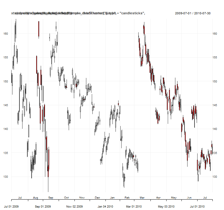
Roughly speaking, cluster one corresponds to a significant up day, cluster two to a significant down day, cluster three to a small up day (although there are a few instances of small down days and neutral days), and cluster four to a small down day (although again there are a few instances of small up days and doji-type candles).
The clusters are not visually perfectly homogeneous. For example, in cluster two there are one or two instances of candles with a large range, but whose overall downwards movement is small. These candles resemble what we know as ‘hammers’ or ‘pins’ in traditional candlestick parlance. Cluster three, while dominated by small up candles, also includes many small down days and hammers/pins. Cluster four is similarly imperfect. My trading experience tells me however that theoretical perfection, while interesting, is an indulgence best left to academic practitioners. I am much more interested in whether the information my research brings to light holds up enough to make a profit.
Part 1 – Clustering patterns
For part one of the analysis, I need a baseline for comparative purposes. The obvious baseline is simply the proportional occurrence of each cluster across the data set. Below is a bar plot describing this (excluding the 2015 data). I’ve added a line graph showing the same information as this will be used for comparative purposes below.
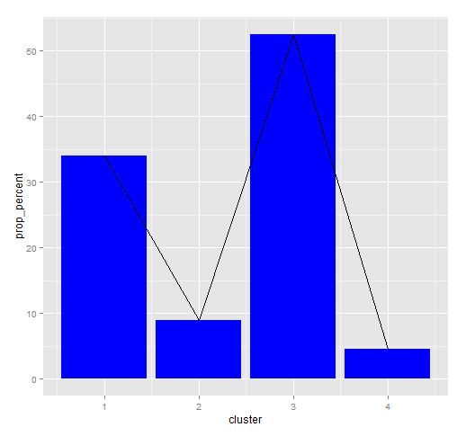
Any lagged clustering patterns will need to be statistically significantly different from these baseline occurrences to be of interest.
To start with, let’s look at the lagged proportional cluster occurrences across the entire data set. In the table below, the columns represent the percentage proportion of each cluster that immediately follows the cluster in the rows (rounded for viewing purposes). This information is reproduced as a series of line graphs in the figure below.
| 1 | 2 | 3 | 4 | |
| 1 | 17 | 15 | 34 | 34 |
| 2 | 20 | 29 | 24 | 28 |
| 3 | 6 | 2 | 57 | 35 |
| 4 | 10 | 3 | 54 | 33 |
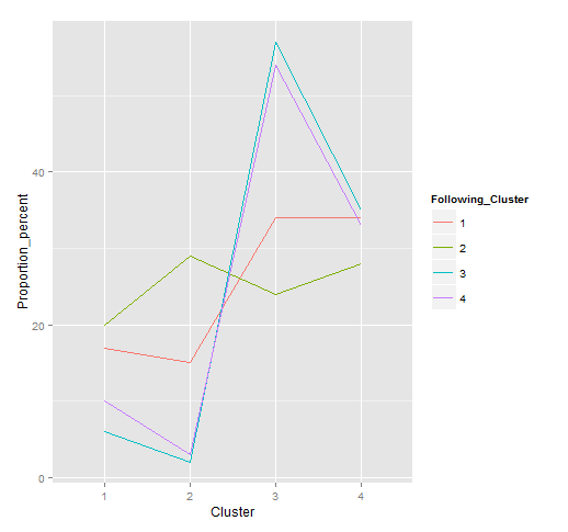
Looking at these results, what can we infer? Some observations that stand out are:
- A big down candle (cluster 2) is repeated in 29% of instances. It is followed by a smaller down candle in 28% of cases. Adding these, we can say that a big down day is followed by another down day 57% of the time.
- A big move in either direction is more often that not preceded by a big move.
- Neutral days or relatively smaller moves also tend to follow each other.
- The patterns of next-cluster proportions are different enough from the sample proportions to warrant further investigation.
I considered investigating the stability of these results with respect to time. For example, it would be possible to set up a moving window on the data set and look at whether these relationships vary across time. However, I’m not sure it would reveal any great insight that is actionable in a practical way. I might come back to this later. For now, lets jump into something more interesting that is more likely to reveal the information I am interested in: returns associated with individual clusters.
Part 2: Returns series analysis
For the second part of the analysis I’ll simply construct a cumulative returns series for a holding period of one day for each cluster. If anything interesting turns up in this analysis, I willl attempt to validate it using my 2015 out of sample data before using it in a trading system. Transaction costs are not included in this analysis.
Here is a chart of the cumulative next day returns for each cluster as well as the cumulative daily returns of the underlying instrument.
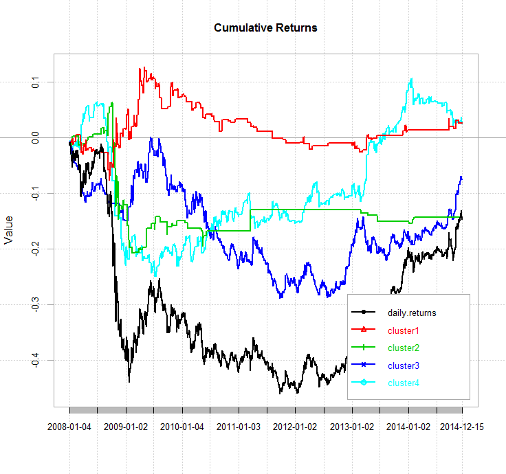
These returns are nothing to get excited about, but a few things stand out. Firstly, the next day returns associated with cluster four significantly out-perform the underlying. More interestingly, it seems to be agnostic to the prevailing trend in the underlying, except for the GFC period. Cluster one also outperforms the underlying, but is somewhat correlated. Cluster two does not contain enough instances to make any useful judgements, and cluster three is highly correlated with the underlying.
Below is the chart of cumulative next day returns for cluster four in the post GFC period from September 2009 (the time when the US government stepped in to rescue Fannie Mae and Freddie Mac). I realise that I am cherry picking from my results, however it does appear that there is value in investigating the performance of cluster four as financial markets adjusted to a new regime.
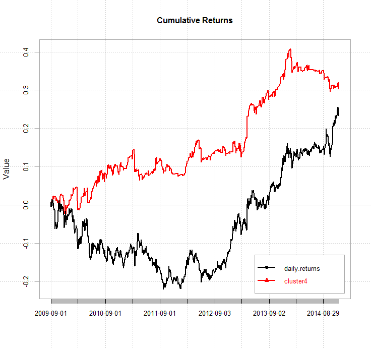
Performance is encouraging. Cluster four out-performs the underlying and does so with a much lower drawdown. However, it would have been impossible to trade this as a system during the period shown since the clusters were identified using that very data. Next, I will investigate cluster four on my out of sample data, which was not used in the cluster identification process.
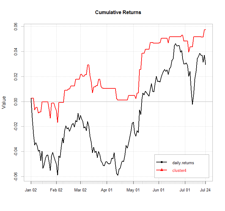
Cluster four out-performs the underlying by a small margin, but it does so with a much more benign drawdown, although its trend-agnosticism seems to have disappeared. The evidence suggests that cluster four has a small but useful predictive utility.
Conclusions and future research directions
I’ve presented a simple application of the k-means clustering algorithm to the prediction of a single financial instrument. I found that the relative values of the daily open, high, low and close appear to have a degree of predictive power for this instrument, particularly in the post-GFC period. These results were validated in an out of sample test. Although gross returns were not spectacular, they were achieved with a much lower drawdown.
A benefit of using an unsupervised learner is that it reduces the chances of over-fitting since there is no optimization on some target value. The trade off is that the information discovered by the learner may have little or no intrinsic utility. In this case, the number of clusters could be an optimization parameter if we varied it and selected the value that resulted in the best returns series.
I used only a small amount of data, made a number of assumptions and applied the approach to just one instrument, chosen at random. There are numerous potential future research directions to take this idea further, including:
- The forex market trades on a 24-hour basis, therefore the choice of daily closing time is somewhat arbitrary. The time used in this analysis was set at 17:00 EST, however a more sensible choice for this particularly market (GBP/JPY) might be 17:00 UTC.
- The approach could be tested on intra-day data, although this would be subject to the vagaries of intra-day volatility cycles which would likely need to be accounted for.
- Other data containing potentially predictive information could also be supplied to the algorithm, for example trend and volatility indicators.
- The analysis could be extended from single candles to two- and three-candle patterns.
- The k-means algorithm is limited in that it requires the user to input the number of clusters before any classification occurs. We could investigate the effect of varying the number of clusters, however hierarchical clustering may provide a better alternative as it does not require any a priori knowledge about the number of clusters into which the data naturally groups.
- Others have suggested the application of a Markov Chain Monte Carlo model in order to build a predictive model based on joint probability tables. This is new territory for me and would require some research into the methodology before I attempted it, however I assume it would require that the joint probabilities were somewhat stable with respect to time, or at least include some means to account for any instability.
- Other markets may or may not be more amenable to this approach.
- Transaction costs should be incorporated into the model.
Here’s the complete R code used in this analysis:
library(fpc)
library(cluster)
library(quantmod)
library(ggplot2)
library(PerformanceAnalytics)
# read in data
data <- read.csv("GBP_JPY.csv", stringsAsFactors = F)
colnames(data) <- c("Date", "GBP_JPY.Open", "GBP_JPY.High", "GBP_JPY.Low", "GBP_JPY.Close") # quantmod requires these names
data$Date <- as.POSIXct(data$Date, format = "%d/%m/%Y")
data <- as.xts(data[, -1], order.by = data[, 1])
data <- data["2008::2014", 1:4] # in-sample data set
chart_Series(data)
# create HLC relative to O
data$HO <- data[,2]-data[,1]
data$LO <- data[,3]-data[,1]
data$CO <- data[,4]-data[,1]
# # K-Means Clustering with clusters based on HO, LO, CO
class_factors <- data[, 5:7]
set.seed(123) # required in order to reproduce results
fit <- kmeans(class_factors,4)
m <- fit$cluster # vector of the cluster assigned to each candle
# which canldes were classifed into each cluster?
cluster <- as.xts(m)
index(cluster) <- index(data) #coerce index of cluster series to match data's index
new_data <- merge.xts(data, cluster)
# plot candles by cluster
chart_Series(xts(coredata(sample_data)[order(sample_data$cluster),],type="candlesticks", order.by = index(sample_data),  theme = chartTheme('black',up.col='green',dn.col='red')))
# count and proportion of each cluster's occurrence in training data
library(plyr)
cluster_count <- count(new_data, vars = "cluster")
cluster_count$prop_percent <- cluster_count$freq*100/sum(cluster_count$freq)
ggplot(cluster_count, aes(x = cluster, y= prop_percent)) + geom_bar(stat = 'identity', fill = 'blue') + geom_line(stat = 'identity', colour = 'black') # plot as bars
# proportaional probability table for next candle
count_table <- table(new_data$cluster , lag(new_data$cluster, 1))
prop_table <- prop.table(table(new_data$cluster , lag(new_data$cluster, 1)), 1) * 100
round(prop_table)
prop_df <- data.frame(round(prop_table))
colnames(prop_df) <- c("Following_Cluster", "Cluster", "Proportion_percent")
ggplot(prop_df, aes(x=Cluster, y=Proportion_percent, group=Following_Cluster)) + geom_line(aes(colour = Following_Cluster))
# returns analysis
new_data$daily_returns <- dailyReturn(new_data)
new_data$cluster1 <- ifelse(new_data$cluster == 1, 1, 0)
new_data$cluster2 <- ifelse(new_data$cluster == 2, 1, 0)
new_data$cluster3 <- ifelse(new_data$cluster == 3, 1, 0)
new_data$cluster4 <- ifelse(new_data$cluster == 4, 1, 0)
cluster1_returns <- lag(new_data$cluster1, 1) * new_data$daily_returns
cluster2_returns <- lag(new_data$cluster2, 1) * new_data$daily_returns
cluster3_returns <- lag(new_data$cluster3, 1) * new_data$daily_returns
cluster4_returns <- lag(new_data$cluster4, 1) * new_data$daily_returns
# comparitive performance of each cluster vs buy and hold
chart.CumReturns(cbind(dailyReturn(new_data), cluster1_returns[-1,], cluster2_returns[-1,], cluster3_returns[-1,], cluster4_returns[-1,]), legend.loc = "bottomright", main = "Cumulative Returns")
# cluster 4 post-GFC
chart.CumReturns(cbind(dailyReturn(new_data["200909::"]), cluster4_returns["200909::",]), legend.loc = "bottomright", main = "Cumulative Returns")
###### apply k-menas to test set (2015)
test_data <- read.csv("GBP_JPY.csv", stringsAsFactors = F)
colnames(test_data) <- c("Date", "GBP_JPY.Open", "GBP_JPY.High", "GBP_JPY.Low", "GBP_JPY.Close") # quantmod requires these names
test_data$Date <- as.POSIXct(test_data$Date, format = "%d/%m/%Y")
test_data <- as.xts(test_data[, -1], order.by = test_data[, 1])
test_data <- test_data["2015", 1:4] #nrow(data), 1:4]
# create HLC relative to O
test_data$HO <- test_data[,2]-test_data[,1]
test_data$LO <- test_data[,3]-test_data[,1]
test_data$CO <- test_data[,4]-test_data[,1]
test_data_kmeans <- data.frame(test_data[, 5:7]) # predict.kmeans seems to be incompatible with xts object
library(DeducerExtras)
test_clusters <- predict.kmeans(fit, data = test_data_kmeans)
test_data$cluster <- test_clusters
test_data$daily_returns <- dailyReturn(test_data)
test_data$cluster4 <- ifelse(test_data$cluster == 4, 1, 0)
cluster4_test_returns <- lag(test_data$cluster4, 1) * test_data$daily_returns
# comparitive performance of cluster 4 vs buy and hold
chart.CumReturns(cbind(dailyReturn(test_data), cluster4_test_returns[-1, ]), legend.loc = "bottomright", main = "Cumulative Returns")


Regarding cluster 4: you picked a good time to start your “outperformance” test, which is basically right after it had its worst drawdown. Yes, the asset did too, I suppose, but nevertheless, I feel like there’s a lot here that’s inconclusive simply due to how little data you used. The GBP_JPY exchange rate should be available for much longer than this period, so I’m hoping you can pursue a way to get another decade of data.
Regarding the findings, it seems that indeed, a massive down day (as defined by the K-means clustering algorithm) seems to have an edge. I suppose intuitively, it’s the idea that right after a major panic sell-off, that the price will take a bounce, and there won’t be as many bad days the next day. Not a particularly bad line of thinking without transaction costs.
Also, regarding “one day after” trading strategies, these sorts of things are the most vulnerable strategies to get hurt by transaction costs, as you might imagine.
Glad to see you using R, but I hope you can find some more data!
Ilya
Thanks for reading and commenting. Yes of course there’s a lot that’s inconclusive. In fact, my “conclusions” section raises more questions and ideas for further research than it draws conclusions!
So you think an additional decade of daily data would be required in order to make any conclusive statements? Is that a rule of thumb or based on some quantitative measure of confidence? In general, I agree that more data is better, with the caveat that any analysis is cognizant of significant market shifts. Obviously, most market inefficiencies seem to have an expiry date, and for this reason I prefer a rolling walk forward analysis to one large training set followed by a single out of sample test. That way, it is possible to observe how a strategy’s edge changes over time. However, it is not my intent to present a robust, complete trading system; rather it is to share some research, garner feedback and hopefully get some new ideas.
In my mind, simply using as much data as possible without the caveat mentioned above is interesting from an academic perspective, but it ignores the practicalities of trading these mostly ephemeral inefficiencies. For example, rather than searching for a universal market truth that holds up in perpetuity (does this even exist?), I would prefer to exploit a shorter-lived inefficiency and use appropriate quantitative risk management to pull out in a timely manner.
Finally, regarding transaction costs. Yes, I know it was remiss of me to exclude these as they are likely to be significant. In your opinion, what’s a simple yet robust way to account for transaction costs in R? I was thinking of simply deducting a fixed amount from the return associated with each trade that mirrors my broker’s average spread and commission, plus an assumption about slippage.
Thanks for the critique. I’m always glad to receive constructive feedback.
Nice article again.
Regarding the need for more data in similar analysis, I like to use proxies to increase the universe available to train the data. For example, it seems reasonable to say that the candle patterns should hold among assets classes in a similar fashion. Take equities for example.
One could train the algorithm on features generated from a bunch of different equity assets. Can we expect the candlestick reaction to a given cluster to be radically different between US and say German equities? I don’t think so, just an avenue to explore.
Personally I am fine with little data when the experiment is carefully crafted and the conclusion drawn are not overly hopeful. I think this passion for large dataset is somewhat restrictive. Sure more data is nice but you have to look at the system. Do you really need a 10 year backtest to be confidant in a system that trades 100x per day? On the other side of the spectrum, would you consider a monthly system for which you see a 3 year backtest? It all depends how long the edge takes to pan out. I think in terms of pattern recognition, it is more important to look at the number of prediction made and accuracy versus length of the backtest.
I apologize for the rant, I just have problems with academic types saying show me more data or your conclusions are invalid. In the real world where people need to make money the hurdle rate is much lower. Much money has been made being the first mover on an anomaly. Why wait for everybody to agree that it’s a good investment opportunity? By that time it’s not nearly as good. Like everything there is tremendous risk/rewards to being the first ones to find something potentially profitable. Concretely, people that found the VXX/XIV trades back in 2007 made an absolute killing in 2008. Back then there was no history to speak of. Look at it now, not a single blog hasn’t proposed a way to capture it. Including the original comment’s author.
Keep up the good work
QF
Fair point regarding VXX/XIV, JP. That said, just about all those methods leave much wanting, including my own methodology (well, that I got from someone else) that completely missed a 27% move in October in XIV.
When you’re using more frequent data, then yes, I agree. But essentially, how do you know the conclusion isn’t simply an artifact of curve-fitting? My issue stems with the fact that this backtest (cluster 4) was started right after it suffered a massive drawdown. Essentially, I like to see longer backtests to see just how bad things can get. For instance, if someone started a backtest on SPY after the GFC and said “look how good this equity curve is! More than a 1 Calmar Ratio just from buying and holding!”
Also, to your point, many XIV/VXX strategies did NOT make a killing in 2008! Quite a few of the ones posted on Volatility Made Simple’s blog actually took obscene drawdowns in 2008 that would have put any fund manager out of business multiple times.
Also, speaking of VXX/XIV trading strategies, I’m wondering if you have anything to add–not necessarily in public. I’m all ears if you wish to collaborate on one.
Ilya, why do you have an issue with the chart showing cluster four’s performance following its drawdown period? In the previous chart, I also show that very drawdown. I am not trying to hold up cluster four as some sort of all powerful predictor of market direction – in fact, I even stated that I am cherry picking the results simply to highlight the interesting observation that its relationship to the underlying appeared to change at around the same time as the world emerged from the GFC. Is my logic in highlighting these observations somehow flawed?
It was not my intention to come across as saying “Look how great this equity curve is!”, and if that’s the way it was interpreted then maybe I need to work on my style. I do however suspect that you are seeking opportunities to inflate your reputation by discrediting the analysis of others. I have no problem with you discrediting my work or the work of others if it is justified. In fact, I welcome the learning opportunity it presents. In this instance however, I feel that you are attributing conclusions to me that I never drew, and then discrediting them. I do have a problem with this as it adds little to the discussion and is something of a waste of time to deal with.
Thanks for the suggestions QF. I hadn’t considered training the algorithm on a bunch of different assets together. Another item to add to the do-do list. It would also be interesting to note any differences between asset classes. For instance, I wonder if currencies would show significantly different behaviour to equities, having accounted for the upwards bias in the latter.
It sounds like we are on the same page regarding the practicalities of market research and systems development. I completely agree that a ‘fit for purpose’ approach is much more useful in designing a system that is intended to be traded. Would I expect my results to be published in a journal of statistical learning? Of course not. And I never intended that. But they do seem to have highlighted a potentially profitable phenomenon. In that sense, the analysis thus far is fit for purpose as far as I’m concerned.
Thanks again for your comments and insights. Always very much appreciated.
Mmm, I did feel that there was a bit of saying “look how good the performance is” regarding the out-of-sample equity curve, or that it even was investigated. I’m highly skeptical of, well, just about any strategy posted online (or anywhere else, for that matter), and try to find the fly in the ointment ASAP. I’ve done this for other authors on my own blog, as well. If you weren’t making a conclusion about outperformance but simply were investigating the OOS equity curve for fun, then mea culpa, but I interpreted it as giving possible praise to a system that may not have warranted it.
Just differences in tolerance, I suppose.
Thanks for that comment Ilya, it was very gracious of you. Regarding the posting of strategies online, rest assured that it is highly unlikely that I’ll post anything that I am actually trading or intend to trade or believe consists of a complete and viable trading system. But please go ahead and pick holes in the methods, results and conclusions that I do post. I welcome the learning opportunity and any robust discussion that comes along with it. I just ask that the discussion is balanced, objective and relevant to the actual content of the post. I’ll work on delivering my conclusions such that they are less open to interpretation.
Anyway, I hope that you keep visiting my blog and commenting on my work. I’ll definitely be an avid reader of yours.
Oh, definitely. I mean, the idea of applying machine-learning methodologies to finance is something that I find highly interesting (as I’ve never seen it done successfully, despite taking Andrew Ng’s machine learning course, and Hastie’s statistical learning). As for not posting complete trading systems, again, respected. That said, my philosophy (at least until recently) has been that anything I think of are things that the institutional investors already know how to do better by virtue of employing multiple PhDs and people with the capability to absorb “write-only” professorially-written theoretical math papers a LOT more quickly than I can, and I’m hoping something I post can be used for inspiration by someone else in the blogosphere to create a better trading system.
Frankly, I’m of the opinion that if the best bloggers on quantocracy worked together, they could probably outperform quite a large amount of the real hedge funds.
That is a fantastic idea. Have you floated it with any of the Quantocracy bloggers? That’s the sort of collaboration I’d be extremely interested in. Have you had much to do with hedge funds and larger institutions? I’ve only had very brief and shallow contact, but what I saw didn’t impress me much at all. I was exposed to a firm that trades using elementary statistics with flawed assumptions combined with technical analysis, and another that trades via discretionary support/resistance/channel type technical analysis. The one thing that did impress me however was how switched on both of these outfits were to risk management. From what I could tell, they spend more time managing risk than analysing the markets. I certainly feel that combining a similar level of risk management with a more robust, statistical approach would lead to significant outperformance – at least of those firms that I referred to.
Interesting read Mr Robot including the debate on when is enough data enough..
From my manual trading experience I would say that sometimes people can focus on perfection when it’s simply not like that and most of the clever people I know fail miserably. Of course there is some science behind this and if your career is maths it will be critical to your success. There are many paths 🙂
Now back to the article. I love the simplicity of kmeans. I am less of a quant and more of a pragmatic programmer with some interests machine learning and fx. I’m only now beginning to attempt to apply ML to fx with a primary focus on evolutionary algorithms and symbolic regression. In part because they are simple…like me :).
I can see a hybrid approach of kmeans to perform simple one bar feature detection and a genetic programming approach to build a multi bar classification or maybe I’ll try some kmeans by itself…
I very much enjoyed the tone of the post and found a quants approach to determining significance enlightening.
Cheers.
Thanks for the comments Sven. I totally agree with your comments about perfection! It recently dawned on me that you don’t need a ‘perfect’ model of the markets in order to make money. A huge part of the art of quantitative development is knowing when to stop developing and start trading. I am still very much getting my head around this.
The simplicity of k-means attracts me to this approach too. Your idea of stacking k-means for feature detection with another supervised learner is an interesting one – another item to add to the ever-expanding to-do list. Would you be interested in collaborating on that idea? In the next few days, I’m going to post a framework for efficiently exploring k-means ideas that I think could be useful in building the first part of the stack.
Hi Mr R,
I’m a complete stranger to R and its magic being heavily Python and traditional c/c++ /web focussed (although I find it increasingly difficult to avoid it as I delve into numpy and scikit/pandas and all the python based R rip offs. )
I’m not sure I can offer much to your stack in knowledge or time but look forward to your next post! You probably have my email feel free to ping me as I’ve always got an opinion and happy to chatter. Cheers.
Hi,
I had a close look at it and found the results quiet interesting. Great article! However, there is one clarification that I would like to make:
In the line number 65 of the code, you have used:
chart.CumReturns(cbind(dailyReturn(new_data), cluster1_returns[-1,], cluster2_returns[-1,], cluster3_returns[-1,], cluster4_returns[-1,]), legend.loc = “bottomright”, main = “Cumulative Returns”)
In relation to this, I believe that an extra argument setting “geometric=FALSE” , should be used because the function chart.CumReturns() internally uses geometric sum and not arithmetic. I suppose, setting it to arithmetic is what will imply a better market analysis rather than calculating geometric sum. And, obviously adding this extra parameter would definitely change the shape of the cumulative curve.
Please clarify this. Thanks!
Hi Amar
Well spotted, thanks for pointing that out!
Cheers
Kris
Hi Kris: Are you still exploring the concepts you shared in this post? Or did you reach a deadend and moved on? I ask because I had a couple of questions for you but if the ultimate result is that the concepts are unproductive, I won’t waste your time. Please let me know. Thanks David
Hi David, to be honest, I never actually gave this the attention it deserved. I didn’t see the research through, because at the time I became distracted with something or other, and I’ve yet to find my way back to it. It’s been on my to-do list for a while. So the short answer is that I never reached a deadend, but I didn’t do enough research to conclude anything positive either.
Hi Team,
I’m new to K-means clustering, is the table shown below the same as the follow-on matrix as mentioned in this tutorial? https://www.quantstart.com/articles/k-means-clustering-of-daily-ohlc-bar-data
1 2 3 4
1 17 15 34 34
2 20 29 24 28
3 6 2 57 35
4 10 3 54 33
Thanks!
Joe
Hey Joe, thanks for reading. I haven’t read that particular article so couldn’t comment. Perhaps another reader could help you out.