In the first Mean Reversion and Cointegration post, I explored mean reversion of individual financial time series using techniques such as the Augmented Dickey-Fuller test, the Hurst exponent and the Ornstein-Uhlenbeck equation for a mean reverting stochastic process. I also presented a simple linear mean reversion strategy as a proof of concept. In this post, I’ll explore artificial stationary time series and will present a more practical trading strategy for exploiting mean reversion. Again this work is based on Ernie Chan’s Algorithmic Trading, which I highly recommend and have used as inspiration for a great deal of my own research.
Go easy on my design abilities…
In presenting my results, I have purposefully shown equity curves from mean reversion strategies that go through periods of stellar performance as well as periods so bad that they would send most traders broke. Rather than cherry pick the good performance, I want to demonstrate what I think is of utmost importance in this type of trading, namely that the nature of mean reversion for any financial time series is constantly changing. At times this dynamism can be accounted for by updating the hedge ratios or other strategy parameters. At other times, the only solution is to abandon the mean reversion approach altogether, perhaps in favour of a trend following approach.
As this post will demonstrate, finding or constructing mean reverting price series is a relatively simple matter. The real key to profitably exploiting such series is the much more difficult matter of understanding, in real time, whether to continue a strategy as is, update its parameters or put it on ice temporarily or permanently.
Let’s get started!
Cointegration
A collection of non-stationary time series variables are said to be cointegrated if there exists a linear combination of those variables that creates a stationary time series. This implies that we can artificially construct a mean reverting time series through the appropriate combination of non-stationary time series. For example, we can construct a portfolio of assets whose market value is a stationary time series and thus amenable to profitable exploitation through mean-reversion techniques, even through the price series of the constituent assets are not themselves mean reverting. A pairs trading strategy, where we buy one asset and short another with an appropriate allocation of capital to each, is an example of this method for exploiting the concept of cointegration, but we can also create more complex portfolios of three or more assets.
We can test whether a given combination of assets forms a stationary process using the stationarity tests described in the previous post. However, it is impossible to know a priori the coefficients (or hedge ratios) that form a stationary portfolio. How then does one test for cointegration? I’ll explore two approaches: the Cointegrated Augmented Dickey-Fuller test and the Johansen test.
Cointegrated Augmented Dickey-Fuller Test
The Cointegrated Augmented Dickey-Fuller Test (CADF test) involves firstly performing a linear regression between two price series to determine the portfolio’s optimal hedge ratio and then conducting a stationarity test on the portfolio’s price series. The example below illustrates this concept using the currencies of Australia and New Zealand since they seem likely to cointegrate given that the economies of both countries are commodity-based and are affected by similar geopolitical forces.
This extends the example in the first post, which explored the mean reverting tendencies of the foreign exchange pair AUD/NZD. In that example, the hedge ratio is always one since equal amounts of AUD and NZD are always being bought and sold. In this example, we allow for a flexible hedge ratio and attempt its optimization. In order to achieve this, we need to introduce a common quote currency, the more liquid the better. It makes sense to choose the US dollar. Therefore, the example below seeks to exploit a stationary portfolio of AUD/USD and NZD/USD.
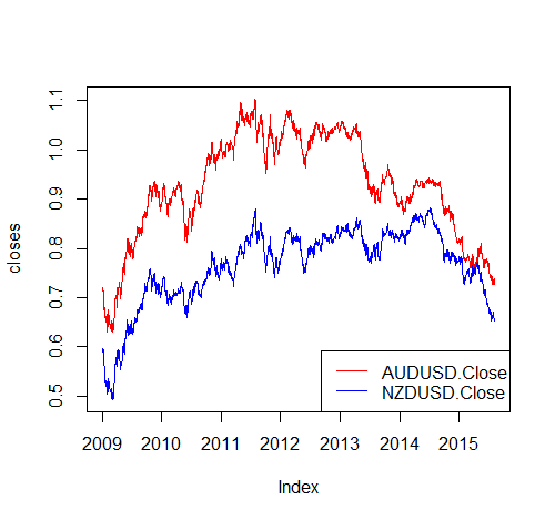
Firstly, the price series of both exchange rates for the period 2009 to mid-2015, which look like they may cointegrate:
A scatter plot further suggests that the price series may cointegrate as the price pairs fall on a roughly straight line:

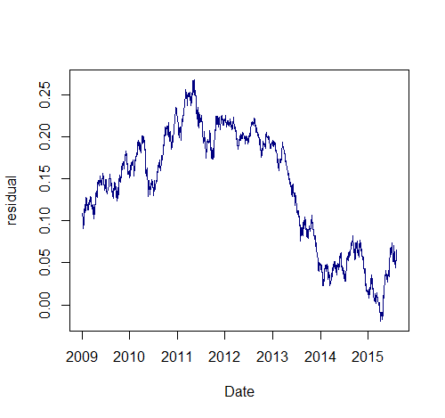
We can use least squares regression to find the optimal hedge ratio and plot the residual of AUD/USD-beta*NZD/USD, which admittedly does not look overly stationary:
## ordinary least squares regression
m <- lm(AUDUSD.Close ~ NZDUSD.Close, data = closes)
beta <- coef(m)[2]
resid <- closes$AUDUSD.Close - beta * closes$NZDUSD.Close
colnames(resid) <- "residual"
plot.zoo(resid, col = 'navyblue', xlab = 'Date', ylab = 'residual')
Next we apply the ADF test to the spread (see the previous post for a brief description of the urca package, and why its implementation of the ADF test is suitable for this application):
## test stationarity of the spread
library(urca)
summary(ur.df(resid, type = "drift", lags = 1))
###############################################
# Augmented Dickey-Fuller Test Unit Root Test #
###############################################
Test regression drift
Call:
lm(formula = z.diff ~ z.lag.1 + 1 + z.diff.lag)
Residuals:
       Min         1Q     Median         3Q        Max
-0.0168356 -0.0022881 -0.0000261  0.0024003  0.0147704
Coefficients:
              Estimate Std. Error t value Pr(>|t|)
(Intercept)  0.0001514  0.0002107   0.719    0.472
z.lag.1     -0.0012629  0.0013435  -0.940    0.347
z.diff.lag   0.0159660  0.0242163   0.659    0.510
Residual standard error: 0.003877 on 1706 degrees of freedom
Multiple R-squared:  0.0007491, Adjusted R-squared:  -0.0004224
F-statistic: 0.6395 on 2 and 1706 DF,  p-value: 0.5277
Value of test-statistic is: -0.94 0.4801
Critical values for test statistics:
      1pct  5pct 10pct
tau2 -3.43 -2.86 -2.57
phi1  6.43  4.59  3.78
In this case, the test statistic we are interested in is -0.94, which is greater than the 10% critical value of -2.57. Therefore, we unfortunately can’t reject the null hypothesis that the portfolio is not mean reverting. However, the negative value of the test statistic indicates that the portfolio is not trending.
One shortcoming of the ordinary least squares approach is that it is asymmetric: switching the dependent and independent variables in the regression results in a different hedge ratio. Good practice would dictate that both options be tested and the arrangement that results in the more negative test statistic be selected. Another approach is to use total least squares regression, which can be used to derive a symmetric hedge ratio. In a geometrical sense, total least squares minimizes the orthogonal distance to the regression line (as opposed to the vertical distance in the case of ordinary least squares) and thus takes into account variance of both the dependent and independent variables. The total least squares solution is easily computed in R using principal component analysis and is not limited to a two-asset portfolio:
## total least squares regression
r <- princomp(~ AUDUSD.Close + NZDUSD.Close, data=closes)
beta_TLS <- r$loadings[1,1] / r$loadings[2,1]
resid_TLS <- closes$AUDUSD.Close - beta_TLS * closes$NZDUSD.Close
colnames(resid_TLS) <- "residual"
plot.zoo(resid_TLS, col = 'blue')
summary(ur.df(resid_TLS, type = "drift", lags = 1))
###############################################
# Augmented Dickey-Fuller Test Unit Root Test #
###############################################
Test regression drift
Call:
lm(formula = z.diff ~ z.lag.1 + 1 + z.diff.lag)
Residuals:
 Min 1Q Median 3Q Max
-0.0253424 -0.0031200 -0.0001321 0.0029981 0.0223268
Coefficients:
 Estimate Std. Error t value Pr(>|t|)
(Intercept) -0.0005211 0.0003666 -1.421 0.155
z.lag.1 -0.0021508 0.0015501 -1.388 0.165
z.diff.lag 0.0174238 0.0241998 0.720 0.472
Residual standard error: 0.005064 on 1706 degrees of freedom
Multiple R-squared: 0.001396, Adjusted R-squared: 0.0002253
F-statistic: 1.192 on 2 and 1706 DF, p-value: 0.3037
Value of test-statistic is: -1.3875 1.0204
Critical values for test statistics:
 1pct 5pct 10pct
tau2 -3.43 -2.86 -2.57
phi1 6.43 4.59 3.78
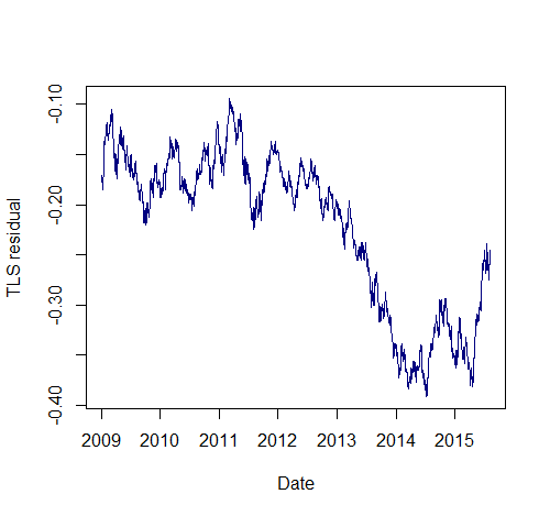
This results in a more negative test statistic and a visually more stationary spread (at least for the period 2009 – 2012, see the figure below), but we are still unable to reject the null hypothesis that the spread obtained through total least squares regression is mean reverting.
Johansen test
The Johansen test allows us to test for cointegration of more than two variables. Recall from the previous post, using a linear model of price changes:
Δy(t) = λy(t − 1) +βt + μ + α1Δy(t − 1) + … + αkΔy(t − k) + εt
where Δy(t) ≡ y(t) − y(t − 1), Δy(t − 1) ≡ y(t − 1) − y(t − 2), etc.
that if λ ≠ 0, then Δy(t) depends on the current level y(t − 1) and therefore is not a random walk. We can generalize this equation for the multivariate case by using vectors of prices y(t) and coefficients λ and α, denoted Y(t), Λ and Α respectively. The Johansen test calculates the number of independent, stationary portfolios that can be formed by various linear combinations of the price series based on the eignevector decomposition of Λ. The urca package contains an implementation of the Johansen test that provides critical values that we can use to test whether we can reject the null hypothesis that there exist 0, 1, 2, …, n-1 cointegrating relationships, where n is the number of constituent time series.
Conveniently, the eigenvectors can be used as the hedge ratios of individual price series to form a stationary portfolio. This process is illustrated below for the AUD/USD-NZD/USD portfolio. A third currency pair – USD/CAD – is added in the next section to attempt to create a stationary portfolio of three currencies.
## johansen test
closes_mat <- cbind(AUDUSD$AUDUSD.Close, NZDUSD$NZDUSD.Close)
jo <- ca.jo(cbind(AUDUSD$AUDUSD.Close, NZDUSD$NZDUSD.Close), type="trace", ecdet="none", K=2) #test trace statistics
print(summary(jo)) # print results of trace statistics
######################
# Johansen-Procedure #
######################
Test type: trace statistic , with linear trend
Eigenvalues (lambda):
[1] 0.004894775 0.001479608
Values of test statistic and critical values of test:
 test 10pct 5pct 1pct
r <= 1 | 2.53 6.50 8.18 11.65
r = 0 | 10.92 15.66 17.95 23.52
Eigenvectors, normalised to first column:
(These are the cointegration relations)
 AUDUSD.Close.l2 NZDUSD.Close.l2
AUDUSD.Close.l2 1.000000 1.0000000
NZDUSD.Close.l2 -3.408877 -0.6886162
Weights W:
(This is the loading matrix)
 AUDUSD.Close.l2 NZDUSD.Close.l2
AUDUSD.Close.d 0.002496743 -9.504283e-05
NZDUSD.Close.d 0.001842973 1.653321e-03
jo2 <- ca.jo(cbind(AUDUSD$AUDUSD.Close, NZDUSD$NZDUSD.Close), type="eigen", ecdet="none", K=2) # eigenvalue test statistics
print(summary(jo2))
In this case, we can’t reject either null hypothesis that r (the number of cointegrating portfolios) is zero or one, since the test statistic in both cases is less than even the 10% critical value. That is, it is unlikely that we can form a stationary portfolio from the price history used in this example. However, it may still be worth pursuing a mean reverting strategy if the half-life of mean reversion is sufficiently low (see the previous post for more details).
As stated above, the eigenvectors form the optimal hedge ratio. They are conveniently ordered by maximum likelihood, so in this case we would select a portfolio of 1 lot of AUD/USD long or short and 3.41 lots of NZD/USD in the opposite direction. In this case, unfortunately, the resulting portfolio does not look any more stationary than that constructed using the ordinary least squares and total least squares regression approaches:

Mean reversion of a portfolio of more than two instruments
We can add a third asset and use the Johansen test to determine the probability that there exists a mean reverting portfolio along with the hedge ratios of such a portfolio. In this case, I will add USD/CAD and take the reciprocal of price so that the quote currencies are consistent (note that when building a trading strategy from this triplet, that the directions signalled for USD/CAD would need to be reversed):
## add third pair to portfolio
USDCAD <- read.csv("USDCAD.csv")
USDCAD <- xts(USDCAD[,-1], as.Date(USDCAD[,1], format="%d/%m/%Y"), src="csv", dateFormat = 'Date')
colnames(USDCAD) <- paste(toupper(gsub("\\^", "", "USDCAD" )),
 c("Open", "High", "Low", "Close", "Volume", "Adjusted"),
 sep = ".")
jo_3_t <- ca.jo(cbind(AUDUSD$AUDUSD.Close, NZDUSD$NZDUSD.Close, 1/USDCAD$USDCAD.Close), type="trace", ecdet="none", K=2)
print(summary(jo_3_t))
jo_3_e <- ca.jo(cbind(AUDUSD$AUDUSD.Close, NZDUSD$NZDUSD.Close, 1/USDCAD$USDCAD.Close), type="eigen", ecdet="none", K=2) #[, 'USDCAD.Close'])
print(summary(jo_3_e))
######################
# Johansen-Procedure #
######################
Test type: maximal eigenvalue statistic (lambda max) , with linear trend
Eigenvalues (lambda):
[1] 0.007006571 0.004775725 0.001302791
Values of teststatistic and critical values of test:
 test 10pct 5pct 1pct
r <= 2 | 2.22 6.50 8.18 11.65
r <= 1 | 8.16 12.91 14.90 19.19
r = 0 | 11.98 18.90 21.07 25.75
Eigenvectors, normalised to first column:
(These are the cointegration relations)
 AUDUSD.Close.l2 NZDUSD.Close.l2 USDCAD.Close.l2
AUDUSD.Close.l2 1.0000000 1.000000 1.000000
NZDUSD.Close.l2 -0.5812779 1.219923 -1.247111
USDCAD.Close.l2 -1.1244247 -1.825102 2.361038
Weights W:
(This is the loading matrix)
 AUDUSD.Close.l2 NZDUSD.Close.l2 USDCAD.Close.l2
AUDUSD.Close.d 0.004438228 -0.004070151 3.141054e-05
NZDUSD.Close.d 0.004877582 -0.002836566 5.746013e-04
USDCAD.Close.d 0.013292047 -0.001652545 3.738115e-06
Again, we unfortunately find no significant cointegrating relationship. However, as discussed in the first post, we sometimes don’t need to hold our results to scientifically stringent statistical significance in order to make money, particularly if the half life of mean reversion is sufficiently short. Therefore, we will retain the first eigenvector to form a portfolio of the three instruments for further investigation. First, let’s take a look at a time series plot of the portfolio’s value:

The half-life of mean reversion of the portfolio is 53.2 days. This is calculated in the same manner as for a single mean reverting time series in the previous post, namely by regressing the value of the portfolio against its value lagged by one time period:
y <- spread3
y.lag <- Lag(y, k=1)
delta.y <- diff(y)
df <- cbind(y, y.lag, delta.y)
df <- df[-1 ,] #remove first row with NAs
regress.results <- lm(delta.y ~ y.lag, data = df)
lambda <- summary(regress.results)$coefficients[2]
half.life <- -log(2)/lambda
print(half.life)
[1] 53.23
Recall that in the previous post, we were able to construct a theoretically profitable linear mean reverting strategy from a single time series with a half life of mean reversion of over 300 days, so at first glance, this result holds some promise.
Linear mean reversion on a cointegrated time series
Below is the equity curve of the linear mean reversion strategy from the previous post on the three-instrument portfolio with the value of the portfolio overlaid on the equity curve:
The strategy suffers significant drawdown and only returns a profit factor of 1.04 and a Sharpe ratio of 0.29.
Obviously, the linear mean reversion strategy presented above and detailed in the previous post would not be suitable for live trading even if the example shown here had generated an impressive backtest. Applied to equities, it would require buying and selling an infinitesimal number of shares when price moves an infinitesimal amount. This is less of a problem when applied to currencies since we can buy and sell in units as small as one-hundredth of a lot. However, the real killer for such a strategy is the trading costs associated with bar-by-bar portfolio rebalancing, as well as the fact that we can’t know the capital required at the outset.
Having said that, there is still much value in testing a mean reversion idea with this linear strategy as it shows whether we can extract profits without any data snooping bias as there are no parameters to optimize. Also, a consequence of the bar-by-bar portfolio rebalancing is that the results of the linear strategy backtest are likely to have more statistical significance than other backtests that incorporate more complex entry and exit rules. Essentially, the simple linear strategy presented here can be used as a proof of concept to quickly determine whether a portfolio is able to be exploited using mean reversion techniques.
A practical approach to linear mean reversion
If the simple linear strategy is not practical for trading, how can we exploit mean reverting portfolios? In Algorithmic Trading, Ernie Chan suggests a Bollinger band approach where trades are entered when price deviates by more than x standard deviations from the mean, where x is a parameter to be optimized. The lookback period for the rolling mean and standard deviation can be optimized or set to the half-life of mean reversion. The trade would be exited when price reverts to y standard deviations from the mean where again y is an optimization parameter. For y = 0 the trade is exited when price reverts to the mean. For y = -x the trade is reversed at x standard deviations from the mean. The obvious advantage of this approach is that we can easily control capital allocation and risk. We can also control the holding period and trade frequency. For example, setting x and y to smaller values will result in shorter holding periods and more round-trip trades.
Exploiting the AUD-NZD-CAD portfolio using this simple implementation with x = 2 and y = 1 returns the following equity curve, with transaction costs included:
The equity curve of the Bollinger strategy is of similar shape to the linear mean reversion strategy, but it trades much less and allows for simpler control of risk and exposure.
Concluding thoughts
This post extended the previous article on the exploitation of individual mean reverting time series by exploring the construction of portfolios whose market value is mean reverting. In addition to the simple linear mean reversion strategy, I also presented a more practical approach that could form the basis of an actual trading strategy.
As stated in the introductory paragraphs, I wanted to show the good and the bad of mean reversion trading. The equity curves presented show periods of outstanding performance as well as periods of the polar opposite. Clearly, there are times when mean reversion is highly profitable, and other times when it just doesn’t work (perhaps trend following is more suitable at these times). But how does one determine, in real-time, which regime to follow? How does one determine when to switch?
I’ve explored several options, including a simple filter based on a trend indicator and a filter based on the actual performance of the strategy in real-time. However, due to the lag associated with the filter values, these approaches are of little if any value. Diversification is another option, that is, continuously trade both mean reversion and trend following strategies at the same time in the belief that the profit from the dominant regime will more than make up for the losses of the other.
If you have an idea about how to address this issue, please let me know in the comments. I’d love to hear from you.
Download files and data used in this analysis
Here you can download the price data and scripts (Zorro and R) used in this post: Mean reversion 2


Knowing when to revert and when to trend follow without the signal lagging is the gazillion dollar question. From my conversations with my mentor, you want a regime changing model for that.
After all, if you have a rangebound instrument, pick your favorite mean reversion indicator and go nuts. If you have a trending market, just buy and hold the trend. But to know which is which? I’d love to see some ideas posted elsewhere. I’ve tried depmix’s default settings and it just gave me garbage.
Regime switching models are a whole new area of research for me. Something I’ve been meaning to tackle for a while now, but haven’t yet gotten around to. This is good motivation to bump it up the to do list. I’ll spend some time learning the first principles and then take a look at the depmix package you mentioned. Although from your experience it sounds like the solution is not a simple one.
Your last suggestion should work fine. Trade a basket of uncorrelated systems with a range of parameters. You’ll get the sum of returns with reduced drawdowns. Some Zorro code is here: https://www.financial-hacker.com/build-better-strategies-part-2-model-based-systems/
Thanks for the suggestion Kevin. I think the key term in your comment is ‘uncorrelated’. I’ve had mixed success with strategy diversification in the past thanks mainly to the correlation between strategies changing over time. But that’s not really a failure of diversification, rather a failure of the trader to properly manage it.
Hi,
great analysis. I did a lot of stuff there and traded (my website is down) so here are some things I found out.
No need to diversify mean reverting and trading, just find 5-10 cointegrating relationship and your Sharpe ratio will be 2+ as residuals are all uncorrelated. You’ll also need to do a WFO or IS/OOS test as no one will take seriously if you have a look-ahead bias. (there is a 50% performance degradation in out of sample testing from my own experience after doing in sample optimization) I strongly suggest WFO for every parameter as it will adapt to changing market modes. Also try other loading from PCA as the first one has the most variance but also the most likely to contain trends.
As for regime switching some filter to filter out trends is an option if you can find one. No need to waste time as regime switching field is huge.
Additional an execution algo that uses EMA vs SMA was better option for me (probably due to large funds using it also and size moves markets), plus you can use 2 st dev to enter but exit after n days could be a better one as a rule.
Anyhow hope it helps .If you want to talk more feel free to contact me.
Kind regards,
D.
Hi D, thanks for sharing your findings! Some great stuff there that hadn’t occurred to me. I’ll definitely be pursuing them. Totally agree regarding walk forward testing; it is an essential part of the evaluation phase of strategy development in my opinion.
I hadn’t considered using the other loadings from the principal components analysis, but I will look into that too. I also like the n-day exit idea. It is appealing in its simplicity and I have found it useful in the past.
Have you tried to use some kind of dominantPhase analysis from Zorro in the cointegrated spread and then trading it (spread) when the phase indicated so?
Ps: I’ve traded cointegrated equity pairs for some 4 yrs, and have no clue about cointegrated fx pairs =) but they do look way better and more robust for doing such.
Hi Eduardo, no I hadn’t considered extracting phase information from the cointegrated spread. My first reaction to the idea is that this approach would be applicable if some sort of cyclical behaviour was present in the spread. I don’t presently know if that is the case or not, but I will certainly look into it. In your experience, have you found exploitable cycles in the spreads you have traded?
Hi there!
Actually, I had this idea when fiddling with the Zorro manual a couple days ago.. I was studying about spectral analysis of financial time series returns and stumble upon Zorro’s cycle/phase indicators based in Hilbert Transforms, so it just occurred to me that, IF you assume that a spread (say, a cointegrated ols residue of two equities) is mean reverting (cointegrated and low enough half life with OU equation), you could probably use the same kind of transformation / cycle analysis that Zorro does (i thinks it’s based in John Ehlers books) in those spreads, in order to get “optimized” entry points, assuming those would predict turning points in the spread itself.
Don’t know if my assumption is mathematically sound, but it’s a hunch..
Personally, I never tried something aside from N*sigmas deviations for trading cointegrated spreads, because of the assumption that they are stochastic.
Sorry for any misspellings,
Best regards
Hi Robot Master,
Thank you for the analysis. One question, is keeping the quote currency constant also necessary for CADF and OU, or it is only for required for Johansen?
Thanks,
Mehmet
If you think about what the tests are doing, the answer to this becomes fairly obvious. The tests mentioned look for a unit root and/or stationarity of the time series in question. In this case, the time series is a spread created by the linear combination of the constituent currency pairs. Would it make much sense to test a spread that consists of, for example:
A*USD/JPY + B*EUR/GBP ???
What would the units of the spread be?
Thank you for answering.
With two pairs with same quote currency, one unit moves have the same dollar values. So what you say is, unless we have this, the tests will not make any sense. Then for example for sgdchf vs zarjpy the pairs to test are sgdusd and zarusd, inverting the quotes or trading signals when necessary.
Am i correct with my interpretation.
Assuming you want to trade a mean reverting spread that consists of SGD and ZAR, yes what you described is how I would approach it.
What about using 10 assets and combining them in groups of 3 with a loop and then calculate the eigenvalues of all those combinantions to get as an output the best cointegration portfolio?
Just a heads up:
You’re missing a negative here:
half.life <- log(2)/lambda
It should be, '-log(2) / lambda'
And caution to the lag function; I'm unsure which package was used, but you might be erroneously shifting the lag forward to y(t+1) by using '-1' if you're using the base:::lag function. I like quantmod:::Lag(y, k = 1).
Best
Hey John
Thanks for pointing that out – you are absolutely correct on both counts. I’ve updated the code accordingly and found that the actual half life should be roughly 53 days, an increase over the 40 days calculated erroneously. I will some day get around to updating the affected results (ie the equity curves of the trading strategies that used the erroneous half life)!
Thanks!
Hi Kris,
Can you enlighten me as to the meaning, when both eigenvalues for a pair are the same sign? They are normally opposite… so I’m selling one and buying the other. The same sign seems to imply go long (or short) on both… which seems at odds with the pair trading methodology.
Thanks,
Hi Kris,
Just came across your blog post while searching for the concept around half-life in mean reversion. I would be keen to know your thoughts around using Kalman filter to estimate hedge ratio. Would be even better if you have an example implementation in R.
Many thanks
riskmaverick
I think Kalman filtering is a great way to estimate hedge ratios. The optimal hedge ratio is rarely static, and Kalman filtering provides a sensible way to update it in real time taking into account the inherent uncertainty in its calculation.
Hi
Is there a easy way to ensure that the cointegration relationship is about to expire?
I’m not sure of any easy way, but one reason these relationships break down is a structural change in the underlying relationship, for example following an earnings announcement that causes a sudden revaluation in one security. In that case, a different cointegrating relationship would probably emerge, once the jump or decline in price settled down to its new level. Another example that relates to the cointegration of ETFs that track the economies of two countries: a relationship could break down when one country’s economy shifts in some fundamental way, for example from a manufacturing to a service base. The two ETFs end up being exposed to different factors and so the cointegration relationship breaks down. In this case, it would happen more slowly.