Rolling and Expanding Windows For Dummies

In today’s article, we are going to take a look at rolling and expanding windows.

By the end of the post,  you will be able to answer these questions:

• What is a rolling window?
• What is an expanding window?
• Why are they useful?

What is a Rolling or Expanding window?

Here is a normal window.

We use normal windows because we want to have a glimpse of the outside, the bigger the window the more of the outside we get to see.

Also as a general rule of thumb, the bigger the windows on someone’s house, the better their stock portfolio did …

Just like real windows, data windows also offer us a small glimpse into something larger.

A moving window allows us to investigate a subset of our data.

Rolling Windows

Often times, we want to know a statistical property of our time series data, but because all of the time machines are locked up in Roswell, we can’t calculate a statistic over the full sample and use that to gain insight.

That would introduce look-ahead bias in our research.

Here is an extreme example of that. Here we’ve plotted the TSLA price and its mean over the full-sample.

import pandas as pd
import matplotlib.pyplot as plt 

#Load TSLA OHLC 
df = pd.read_csv('TSLA.csv')

#Calculate full sample mean
full_sample_mean = df['close'].mean()

#Plot
plt.plot(df['close'],label='TSLA')
plt.axhline(full_sample_mean,linestyle='--',color='red',label='Full Sample Mean')

plt.legend()
plt.show()

 

In this case, if we just bought TSLA when the price was under the mean and Sold it above the mean, we would have made a killing, well at least up to 2019…

But the problem is that we wouldn’t have known the mean value at that point in time.

So it’s pretty obvious why we can’t use the entire sample, but what can we do then? One way we could approach this problem is by using rolling or expanding windows.

If you’ve ever used a Simple Moving Average, then congratulations – you’ve used a rolling window.

How do rolling windows work?

Let’s say you have 20 days of stock data and you want to know the mean price of the stock for the last 5 days. What do you do?

You take the last 5 days, sum them up and divide by 5.

But what if you want to know the average of the previous 5 days for each day in your data set?

This is where rolling windows can help.

In this case, our window would have a size of 5, meaning for each point in time it contains the mean of the last 5 data points.

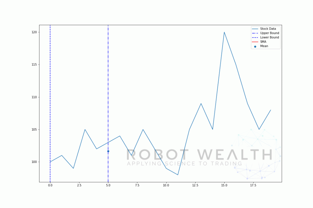
Let’s visualize an example with a moving window of size 5 step by step.

#Random stock prices
data = [100,101,99,105,102,103,104,101,105,102,99,98,105,109,105,120,115,109,105,108]

#Create pandas DataFrame from list
df = pd.DataFrame(data,columns=['close'])

#Calculate a 5 period simple moving average
sma5 = df['close'].rolling(window=5).mean()

#Plot
plt.plot(df['close'],label='Stock Data')
plt.plot(sma5,label='SMA',color='red')

plt.legend()
plt.show()

 

So let’s breakdown this chart.

• We have 20 days of stock prices in this chart, labelled Stock Data.
• For each point in time (the blue dot) we want to know what’s the 5 day mean price.
• The stock data used for the calculation is the stuff between the 2 blue vertical lines.
• After we calculate the mean from 0-5 our mean for day 5 becomes available.
• To get the mean for day 6 we need to shift the window by 1 so, the data window becomes 1-6.

And this is what’s known as a Rolling Window, the size of the window is fixed. All we are doing is rolling it forward.

As you have probably noticed we don’t have SMA values for points 0-4. This is because our window size (also known as a lookback period) requires at least 5 data points to do the calculation.

Expanding Windows

Where rolling windows are a fixed size, expanding windows have a fixed starting point, and incorporate new data as it becomes available.

Here’s the way I like to think about this:

“What’s the mean of the past n values at this point in time?” – Use rolling windows here.

“What’s the mean of all the data available up to this point in time?” – Use expanding windows here.

Expanding windows have a fixed lower bound. Only the upper bound of the window is rolled forward (the window gets bigger).

Let’s visualize an expanding window with the same data from the previous plot.

#Random stock prices 
data = [100,101,99,105,102,103,104,101,105,102,99,98,105,109,105,120,115,109,105,108] 

#Create pandas DataFrame from list 
df = pd.DataFrame(data,columns=['close']) 

#Calculate expanding window mean
expanding_mean = df.expanding(min_periods=1).mean()

#Calculate full sample mean for reference
full_sample_mean = df['close'].mean()

#Plot 
plt.plot(df['close'],label='Stock Data') 
plt.plot(expanding_mean,label='Expanding Mean',color='red')
plt.axhline(full_sample_mean,label='Full Sample Mean',linestyle='--',color='red')


plt.legend()
plt.show()

 

You can see that in the beginning, the SMA is a bit jittery. That’s because we have a smaller number of data points at the beginning of the plot, and as we get more data, the window expands until eventually the expanding window mean converges to the full sample mean, because the window has reached the size of the entire data set.

Summary

It is important not to use data from the future to analyse the past. Rolling and expanding windows are essential tools to help “walk your data forward” to avoid these issues.

If you liked this you’ll probably like these too…

Financial Data Manipulation in dplyr for Quant Traders

Using Digital Signal Processing in Quantitative Trading Strategies

Backtesting Bias: Feels Good, Until You Blow Up