
- do the best job possible of designing and building their trading strategy to be robust to a range of future market conditions
- chill out and let the strategy do its thing, understanding that drawdowns are business-as-usual
- go and look for other opportunities to trade.
What is Drawdown in Trading?
Drawdown is just a fancy word for the fall from a peak in your equity curve to the next low point. Traders usually quote it as a percentage, and it tells you how much of your capital has been eroded before things recover. Why does it matter? Because drawdowns are inevitable. They’re the tax we all pay for pursuing returns in noisy, efficient markets. The deeper or longer the drawdown, the harder it is on both your capital and your psychology. Every strategy, no matter how well researched, will go through periods of drawdown. The real question isn’t if they happen, but whether what you’re experiencing is still “normal” or if your strategy has actually broken down. That’s exactly the problem the Cold Blood Index is designed to help with.Becoming Cold-Blooded….
Johan Lotter, the brains behind the Zorro development platform, proposed an empirical approach to the problem of reconciling backtest returns with live returns. Put simply, his approach compares a drawdown experienced in live trading to the backtested equity curve, and he called this approach the Cold Blood Index (CBI). Apart from sounding like something you’d use to rank your favourite reptiles, we’re going to break down the CBI and find out what it can tell you about your drawdowns in live trading — especially when panic alarms are busy going off in your lizard brain. You can see Johan’s blog post from 2015 for the original article.
Let’s break it down….
You can see Johan’s blog post from 2015 for the original article.
Let’s break it down….
The Cold Blood Index Explained
Paying homage to its creator, we’ll utilise Zorro to illustrate the CBI in action. Don’t worry if any of these details are hard to grasp. Follow the bigger picture and revisit the finer nuances later. Say you have been trading a strategy live for (t) days and are in a drawdown of length (l) and depth (D). You want to know how this compares with the backtest. Most people will want to use this to decide whether their strategy is ‘broken’, but remember that backtests are far from a 100% accurate representation of future performance. So be careful how you use this thing. The CBI is an estimate of the probability of experiencing the current drawdown if the strategy hasn’t deviated from its backtest.- A high CBI indicates that the current drawdown is not unexpected, meaning the strategy probably hasn’t deviated from its backtest.
- A low CBI indicates that the system that produced the backtest is very unlikely to have produced the current drawdown – meaning the live strategy has deviated from the backtest.
Example: Underwater from Day One
Naturally, let’s start with the worst-case scenario. Take the simple case where our trading time, (t) is the same as the length of our current drawdown, (l). To calculate the empirical distribution, we simply take a window of length (l) and place it at the first period in the backtest balance curve. That is, the window initially covers the backtest balance curve from the first bar to bar (l). Then, we simply calculate the difference in balance across the window, (G), and record it. Then, we slide the window by one period at a time until we reach the end of the balance curve, calculating the change in balance across each window as we go. At the completion of this process, we have a total of (M) values for balance changes across windows of length (l) ((M) is equal to the length of the backtest minus (l) plus one). Of these (M) values, (N) will show a greater drawdown than our current drawdown, (D). Then, the CBI, here denoted (P), is simply [P = \frac{N}{M}] Here’s the code for calculating the CBI and plotting the empirical distribution from the backtest, for this special case where the strategy is underwater from the first day of live trading:/* Cold Blood Index
Special case of drawdown length equal to trade time
That is, strategy underwater since inception
*/
int TradeDays = 60; // Days since live start and in drawdown
var DrawDown = 20; // Current drawdown depth in account currency
string BalanceFile = "Log\\simple_portfolio.dbl";
void Histogram(string Name,var Value,var Step,int Color)
/* plots a histogram given a value and bin width */
{
var Bucket = floor(Value/Step);
plotBar(Name,Bucket,Step*Bucket,1,SUM+BARS+LBL2,Color);
}
void main()
{
var HistStep = 10; //bin width of histogram
plotBar("Live Drawdown",DrawDown/HistStep,DrawDown,80,BARS|LBL2,BLACK); //mark current drawdown in histogram
// import balance curve
int CurveLength = file_length(BalanceFile)/sizeof(var);
var *Balances = file_content(BalanceFile);
// get number of samples
int M = CurveLength - TradeDays + 1;
// sliding window calculations
var GMin=0, N=0; //define N as a var to prevent integer truncation in calculation of P
int i;
for(i=0; i<M; i++)
{
var G = Balances[i+TradeDays-1] - Balances[i];
if(G <= -DrawDown) N += 1.;
if(G < GMin) GMin = G;
Histogram("G", G, HistStep, RED);
}
var P = N/M;
printf("\nTest period: %i days",CurveLength);
printf("\nWorst test drawdown: %.f",-GMin);
printf("\nSamples: %i\nSamples worse than observed: %i",M,(int)N);
printf("\nCold Blood Index: %.1f%%",100*P);
}
To use this script, you first need to save the profit and loss time series data from a backtest (also, the backtest will need to use the same money management approach as used in live trading).
Do that by setting Zorro’s LOGFILE and BALANCE parameters, which automatically save the backtest’s balance curve in Zorro’s log file.
Having saved the balance curves, in the CBI script above, make sure the string BalanceFile is set correctly (line 11).
Here’s an example. Say we had been trading our strategy live and we were concerned about the performance of the EUR/USD: rsi component. It’s been trading for 60 days now, and that component is showing a drawdown of $20.
Plugging those values into the script above and loading that component’s backtested balance curve gives the following histogram:
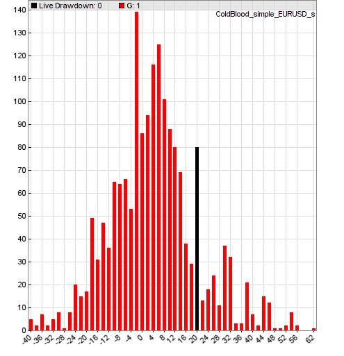 The script also outputs to the Zorro GUI window some pertinent information. Firstly, that of 1,727 sample windows, 73 were worse than our observed drawdown. CBI is then calculated as (73/1,727 = 0.04), which may exceed some individuals’ threshold confidence level of 0.05 (remember a smaller CBI provides stronger evidence of a “broken” strategy). But this is somewhat arbitrary.
We can also run the CBI script with various values of TradeDays and DrawDown to get an idea of what sort of drawdown would induce changes in the p-value.
The script also outputs to the Zorro GUI window some pertinent information. Firstly, that of 1,727 sample windows, 73 were worse than our observed drawdown. CBI is then calculated as (73/1,727 = 0.04), which may exceed some individuals’ threshold confidence level of 0.05 (remember a smaller CBI provides stronger evidence of a “broken” strategy). But this is somewhat arbitrary.
We can also run the CBI script with various values of TradeDays and DrawDown to get an idea of what sort of drawdown would induce changes in the p-value.
And when a profitable strategy starts to sink?
The implementation of CBI above is for the special case where the strategy has been experiencing a drawdown since the first day of live trading. Of course, this (hopefully) won’t always be the case! For drawdowns that come after some new equity high, calculation of the empirical distribution is a little tricker. Why? Because we now have to consider the total trading time (t) as well as the drawdown time (l). Reproducing this distribution of drawdowns faithfully would require traversing the balance curve using nested windows: an outer window of length (t) and an inner window of length (l) traversing the outer window, period by period, at every step of the outer window’s journey across the curve. That is, for a backtest of length (y), we now have ((y-t+1)*(t-l+1)) windows to evaluate. Rather than perform that cumbersome operation, we can apply the same single rolling window process that was used in the simple case, combined with some combinatorial probability to arrive at a formula for CBI, which we denote (P), in terms of the previously defined parameters (M, N, T): [P = 1 – \frac{(M – N)!(M – T)!}{M!(M – N – T)!}] The obvious problem with this equation is that it potentially requires evaluation of factorials on the order of ((10^3)!), which is approximately (10^{2500}), far exceeding the maximum range of var type variables. To get around that inconvenience, we can take advantage of the relationships [ln(1000 * 999 * 998 * … * 1) = ln(1000) + ln(999) + ln(998) + … + ln(1)] and [e^{ln(x)} = x] to rewrite our combinatorial equation thus: [P = 1 – e^{x}] where [x = ln(\frac{(M – N)!(M – T)!}{M!(M – N – T)!}] [= ln((M – N)!) + ln((M – T)!) – ln(M!) – ln((M – N – T)!)] Now we can deal with those factorials using a function that recursively sums the logarithms of their constituent integers, which is much more tractable. Here’s a script that verifies the equivalence of the two approaches for small integers, as well as its output:var logsum(int n)
{
if(n <= 1) return 0;
else return log(n)+logsum(n-1);
}
int factorial(int n)
{
if (n <= 1) return 1;
if (n >= 10)
{
printf("%d is too big", n);
return 0;
}
return n*factorial(n-1);
}
void main()
{
int M = 5;
int N = 3;
printf("\nEvaluate x = (%d-%d)!/%d!using\nfactorial and log transforms", M, N, M);
printf("\nBy evaluating factorials directly,\nx = %f", (var)factorial(M-N)/factorial(M));
printf("\nBy evaluating sum of logs,\nx = %f", exp(logsum(M-N) - logsum(M)));
}
/* OUTPUT:
Evaluate x = (5-3)!/5!using
factorial and log transforms
By evaluating factorials directly,
x = 0.016667
By evaluating sum of logs,
x = 0.016667
*/
Here’s the script for the general case of the CBI (courtesy Johan Lotter):
/* Cold Blood Index

General case of the CBI where DrawDownDays != TradeDays

*/

int TradeDays = 100; // Days since live start
int DrawDownDays = 60; // Length of drawdown
var DrawDown = 20;   // Current drawdown depth in account currency

string BalanceFile = "Log\\simple_portfolio.dbl";

var logsum(int n)
{
    if(n <= 1) return 0;
    else return log(n)+logsum(n-1);
}

void main()
{
    // import balance curve
    int CurveLength = file_length(BalanceFile)/sizeof(var);
    var *Balances = file_content(BalanceFile);

    // calculate parameters and check sufficient length
    int M = CurveLength - DrawDownDays + 1;
    int T = TradeDays - DrawDownDays + 1;

    if(T < 1 || M <= T) {
        printf("Not enough samples!");
        return;
    }

    // sliding window calculations
    var GMin=0, N=0; //define N as a var to prevent integer truncation in calculation of P
    int i = 0;
    for(; i < M; i++)
    {
        var G = Balances[i+DrawDownDays-1] - Balances[i];
        if(G <= -DrawDown) N += 1.;
        if(G < GMin) GMin = G;
    }

    var P;
    if(TradeDays > DrawDownDays)
        P = 1. - exp(logsum(M-N)+logsum(M-T)-logsum(M)-logsum(M-N-T));
    else
        P = N/M;

    printf("\nTest period: %i days",CurveLength);
    printf("\nWorst test drawdown: %.f",-GMin);
    printf("\nM: %i  N: %i  T: %i",M,(int)N,T);
    printf("\nCold Blood Index: %.1f%%",100*P);
}
Using the same drawdown length and depth as in the simple case, but now having traded for a total of 100 days, our new CBI value is 83%, which provides no evidence to suggest that the component has deteriorated.
The Resampled Cold Blood Index
For comparing drawdowns in live trading to those in a backtest, the CBI is useful. But we can do better by incorporating statistical resampling techniques. Drawdown is a function of the sequence of winning and losing trades. However, a backtest represents just one realization of the numerous possible winning and losing sequences that could arise from a trading system with certain returns characteristics. As such, the CBI presented above considers just one of many possible returns sequences that could arise from a given trading system. So, we can make the CBI more robust by incorporating the algorithm into a Monte Carlo routine, such that many unique balance curves are created by randomly sampling the backtested trade results, and running the CBI algorithm separately on each curve. The code for this Resampled Cold Blood Index is shown below, including calculation of the 5th, 50th and 95th percentiles of the resampled CBI values./* Resampled Cold Blood Index
General case of the Resampled CBI where DrawDownDays != TradeDays
*/
int TradeDays = 100; // Days since live start
int DrawDownDays = 60; // Length of drawdown
var DrawDown = 20; // Current drawdown depth in account currency
string BalanceFile = "Log\\simple_portfolio.dbl";
var logsum(int n)
{
if(n <= 1) return 0;
else return log(n)+logsum(n-1);
}
void main()
{
int CurveLength = file_length(BalanceFile)/sizeof(var);
printf("\nCurve Length: %d", CurveLength);
var *Balances = file_content(BalanceFile);
var P_array[5000];
int k;
for (k=0; k<5000; k++)
{
var randomBalances[2000];
randomize(BOOTSTRAP, randomBalances, Balances, CurveLength);
int M = CurveLength - DrawDownDays + 1;
int T = TradeDays - DrawDownDays + 1;
if(T < 1 || M <= T) {
printf("Not enough samples!");
return;
}
var GMin=0., N=0.;
int i=0;
for(; i < M; i++)
{
var G = randomBalances[i+DrawDownDays-1] - randomBalances[i];
if(G <= -DrawDown) N += 1.;
if(G < GMin) GMin = G;
}
var P;
if(TradeDays > DrawDownDays)
P = 1. - exp(logsum(M-N)+logsum(M-T)-logsum(M)-logsum(M-N-T));
else
P = N/M;
// printf("\nTest period: %i days",CurveLength);
// printf("\nWorst test drawdown: %.f",-GMin);
// printf("\nM: %i N: %i T: %i",M,(int)N,T);
// printf("\nCold Blood Index: %.1f%%",100*P);
P_array[k] = P;
}
var fifth_perc = Percentile(P_array, k, 5);
var med = Percentile(P_array, k, 50);
var ninetyfifth_perc = Percentile(P_array, k, 95);
printf("\n5th percentile CBI: %.1f%%",100*fifth_perc);
printf("\nMedian CBI: %.1f%%",100*med);
printf("\n95th percentile CBI: %.1f%%",100*ninetyfifth_perc);
}
Using the same drawdown length, drawdown depth and trade time as we evaluated in the single-balance curve example, we now find that our median resampled CBI is around 98%.
It turns out that the value obtained by only evaluating the backtest balance curve was closer to the 5th percentile (that is, the lower limit) of resampled values.
While this is not significant in this example (regardless of the method used, it is clear that the component has not deteriorated) this could represent valuable information if things were more extreme.
The usefulness of the resampled CBI declines for increasing backtest length, but it is easily implemented, comes at little additional compute time (thanks in part to Lite-C’s blistering speed), and provides additional insight into strategy deterioration by considering the random nature of individual trade results.
Note however that this method would break down in the case of a strategy that exhibited significant serially correlated returns, since resampling the backtest balance curve would destroy those relationships.
Could we use this to automate our decision to retire strategies?
As interesting as this approach is, probably not…. In nearly all cases this is giving the right answer to the wrong question:“Should I pull out of this strategy bdcause its live performance looks different to the backtest?”To labour the points we made in the first post in this series, experienced traders know that it’s a bad idea to set performance expectations based on a backtest. Manageable deviations from that backtest performance usually won’t trigger any alarm bells that inspire interference with the strategy. Instead, we make tea and look for other trades. To succeed in trading you have to realise and accept the randomness and efficiency of the markets — part of which means sitting through rather uncomfortable drawdowns which won’t show up in R&D. Being disappointed by live performance vs your exciting backtest is very much the norm…. you just have to take it on the chin and trust the soundness of your development process. The markets are too efficient and chaotic to care about meeting our expectations.
We call this “Embracing the Mayhem”.
Embracing the Mayhem is just one of the 7 Trading Fundamentals we teach inside our Bootcamps. These Fundamentals show the approach we use to trade successfully with Robot Wealth, which is normally only learned after years of expensive trial, error and frustration. But you can skip all that — you can get access to a bunch of these Fundamental videos for free by entering your email below:Free Case Study:
A wantaway engineer’s journey into professional trading and out again
I went from engineering to an equity partnership at a prop trading firm to running my own systematic trading operation from home in Western Australia.
This case study is the full story – every mistake, every breakthrough, and some things I trade today.


