An easy, practical way to harness an edge in the face of trading costs is the “no trade region” technique.
It nearly always improves after-cost performance. Here’s a real example:
And it does so with only one-tenth of the trading of the baseline strategy!
Uncertain edge vs certain costs
A good thing to remember is that your edge is uncertain – not only do you usually not know how big it is, you also don’t know if it even exists anymore.
On the other hand, your trading costs are certain. Every time you click “buy” or “sell,” you’re paying for the privilege.
One of the most powerful improvements to any strategy is simply trading less. Or more accurately, doing the bare minimum amount of trading required to harness your edge.
The no-trade region: A powerful heuristic
Here’s how it works:
Your strategy generates a target position (\(w\)) for each asset. But instead of immediately trading to that exact position, you create a buffer zone (\(b\)) around it. For a minimum commission cost structure (where there is some fixed minimum commission):
- If your current position (\(w_0\)) is below \(w-b\), trade up to \(w\)
- If your current position is above \(w+b\), trade down to \(w\)
- If your position falls within this “no trade region,” do nothing
If your costs are only a function of size, you would trade to the edge of the barrier instead:
- If your current position (\(w0\)) is below \(w-b\), trade up to \(w-b\)
- If your current position is above \(w+b\), trade down to \(w+b\)
- If your position falls within this “no trade region,” do nothing
Express \(b\) as a percentage of your target weight.
This simple rule dramatically reduces unnecessary churn while still keeping you reasonably aligned with your strategy’s intentions.
How big should your no-trade region be?
The simplest approach is to run a bunch of simulations and find the value that maximises after-cost Sharpe ratio.
This might sound like overfitting, but so long as you think carefully about what you’re doing, it’s not a huge deal. It’s certainly not on the same level as fitting a trend rule to the 127-day moving average!
However, a sensible way to view a backtest is that it likely overstates performance. Like it or not, some sort of bias will usually creep into the development process. I therefore view any backtest as an absolute upper limit on expected performance going forward.
The implication is that optimising the buffer value on backtested Sharpe will produce a value that is too low, since the backtest is a little overestimated. So it’s not a bad idea to increase the value of the buffer over what you found in your backtest.
I’ve heard of people doubling this value; personally, I might add, say 25-50% – but it depends on what you’re doing. In any event, it’s useful to remember that we’re not trying to be overly precise (we can’t be) – we’re just trying to reduce our trading costs to the extent possible.
This simple technique can have quite an impact. While it isn’t an edge in itself, it can help you harness edges that would otherwise not survive trading costs and put more money in your pocket from edges that would.
An example
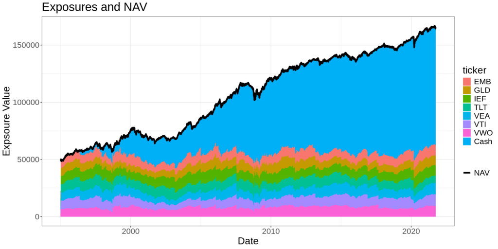
This is a simulation of a 7-asset, equal-weight, risk-premia harvesting strategy.
It simply distributes $50k across 7 ETFs in equal dollar amounts. It doesn’t reinvest any profits; it simply allows the cash balance to grow over time. The simulated costs correspond to an Interactive Brokers tiered commission structure.
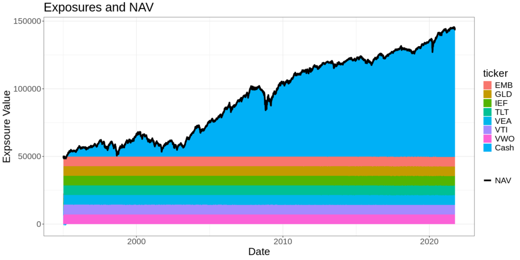
The colours represent the exposure to each asset in the portfolio. The blue represents the cash balance, which grows over time as the value of the underlying assets goes up. You can see that the asset exposures are rebalanced back to equal dollar weight daily.
The after-cost Sharpe was about 0.7, and the trading costs were over 10% of the strategy’s profits.
It turned over about 50% of the portfolio value per year, on average (which might not be a lot for an alpha trade, but feels excessive for a risk premia harvesting strategy).
Here’s a plot of commissions per asset over time:
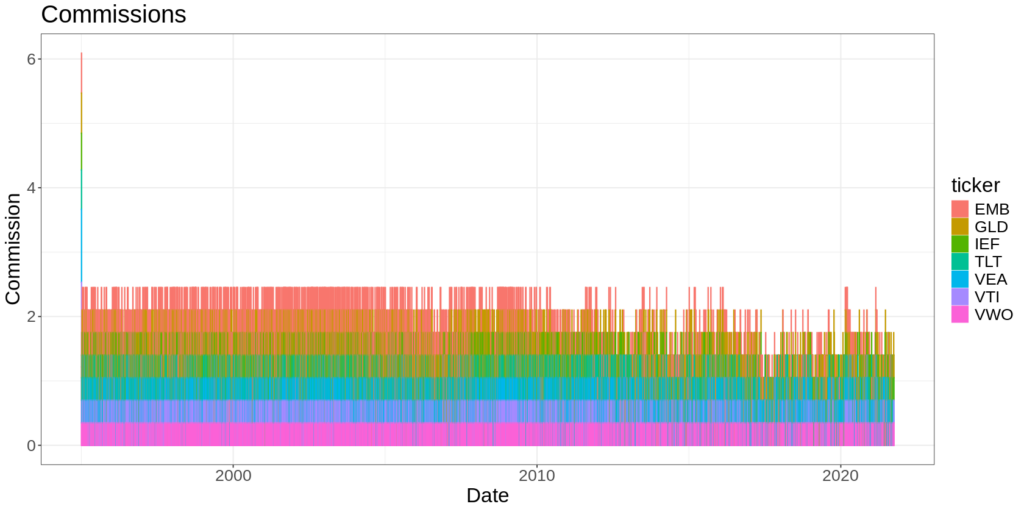
You can see that it’s trading and paying costs pretty much every day.
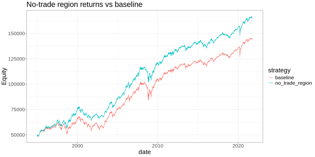
If you run a bunch of backtests using different values for the barrier, you get the following plot of the after-cost Sharpe:
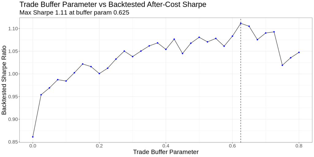
For the sake of the example, let’s increase the trade barrier to 0.5 – the point where after-cost Sharpe starts to level off.
(In reality, you could probably go even higher – the trade-off would be a higher tracking error, but even less trading.)
This results in a higher after-cost Sharpe (0.9 vs 0.7), higher total return, and much lower turnover (5% vs 50% per year).
The trade-off is the large tracking error. You can see that our asset weights deviate quite far from equality, whereas when we rebalanced every day, they were virtually constant.
Of course, in this case, for the trader who cares about making money in the most efficient way possible, you’d take this trade-off every day of the week.
If you were an ETF manager managing to a mandate, your take on the trade-off would be quite different.
Another interesting point is the dynamics of the minimum commission structure. If your account is small, you’ll hit these minimum commissions more often, and your commissions will be higher as a proportion of your capital.
In that case, you’d prefer to do as little trading as possible, and your preferred trade barrier would be even higher.
I used rsims to do the backtests and make the plots. It’s an R library for backtesting that I wrote to fit in with my typical workflow. I added the code for this example to the github repo here if you’d like to explore it further.
Summary
- Trading costs are guaranteed, while your trading edge is uncertain and difficult to measure.
- The “no-trade region” can reduce trading costs by creating a buffer around your target position. You only trade when your actual position moves outside this buffer.
- This helps you do only the minimum amount of trading required to harness your edge.