What if you had a tool that could help you decide when to apply mean reversion strategies and when to apply momentum to a particular time series? That’s the promise of the Hurst exponent, which helps characterise a time series as mean reverting, trending, or a random walk. For a brief introduction to Hurst, including some Python code for its calculation, check out our previous post. Even if you have read this post previously, it is worth checking out again as we have updated our method for calculating Hurst and believe this new implementation is more accurate.
Challenges of Applying Hurst to Financial Data
It would be great if we could plug some historical time series data into the Hurst algorithm and know whether we expect the time series to mean revert or trend. But as is usually the case when we apply such tools to the financial domain, it isn’t quite that straightforward. In the last post, we noted that Hurst gives different results depending on how it is calculated; this begs the question of how to choose a calculation method intelligently so that we avoid choosing arbitrary parameters. The purpose of this post is to delve into the algorithm behind the calculation of Hurst in an attempt to understand this very question. Hopefully we will draw some conclusions around if, when and how we might apply the very attractive theory of Hurst in a manner that is practical to systematic traders.
Using Python for Hurst Analysis
In this post, we perform the analysis in Python, which is something of a departure from tradition for Robot Wealth. We are currently building our skills in both Python and the Microsoft .Net framework to complement our skills in R, C and MATLAB, so expect to see more from us using these tools.</p></p>
Introduction to Hurst
The Hurst exponent, H, measures the long-term memory of a time series, characterising it as either mean-reverting, trending or a random walk. H is a number between 0 and 1, with H < 0.5 indicating mean reversion, H > 0.5 indicating a trending time series and H = 0.5 indicating a random walk. Smaller and larger values of H indicate stronger mean-reversion and trending, respectively.
Here, we apply the algorithm for calculating Hurst from the previous post to an artificial mean-reverting time series created from a discrete Ornstein-Uhlenbeck process parameterised arbitrarily:
# create OU process
N = 100000
ts = zeros(N)
mu = 0.75
theta = 0.04
sigma = 0.05
for i in range(1,N):
    dts  = (mu - ts[i-1])*theta + randn()*sigma
    ts[i] = ts[i-1] + dts
# calculate Hurst
lag1 = 2
lags = range(lag1, 20)
tau = [sqrt(std(subtract(ts[lag:], ts[:-lag]))) for lag in lags]
plot(log(lags), log(tau)); show()
m = polyfit(log(lags), log(tau), 1)
hurst = m[0]*2
print 'hurst = ',hurst
This returns a Hurst exponent of around 0.43, indicating that the series is moderately mean reverting, as expected.
As the algorithm shows, calculation of Hurst is related to the autocorrelations of the time series. Autocorrelation (also known as serial correlation) refers to the correlation between a time series and lagged values of itself. In particular, Hurst is related to the rate at which these autocorrelations decrease as the lag increases. We know that we get different values of Hurst depending on which lags we use in its calculation. So which lags should we focus on?
Analysing SPY with Hurst
In the example above, we used lags 2-20. This is completely arbitrary and is the same value used by default in the MATLAB genhurst function for calculating the Hurst exponent. Let’s look at some real financial data – price history for the SPY ETF – and investigate the effect of varying this range of lags and the subset of data analysed. Here’s the code for obtaining and plotting the data:
import pandas.io.data as web
import datetime
from numpy import *
from pylab import plot, show
start = datetime.datetime(1993, 1, 1)
end = datetime.datetime(2016, 12, 31)
spy = web.DataReader("SPY", 'yahoo', start, end)
closes = spy['Adj Close'][:]
plot(closes); show()
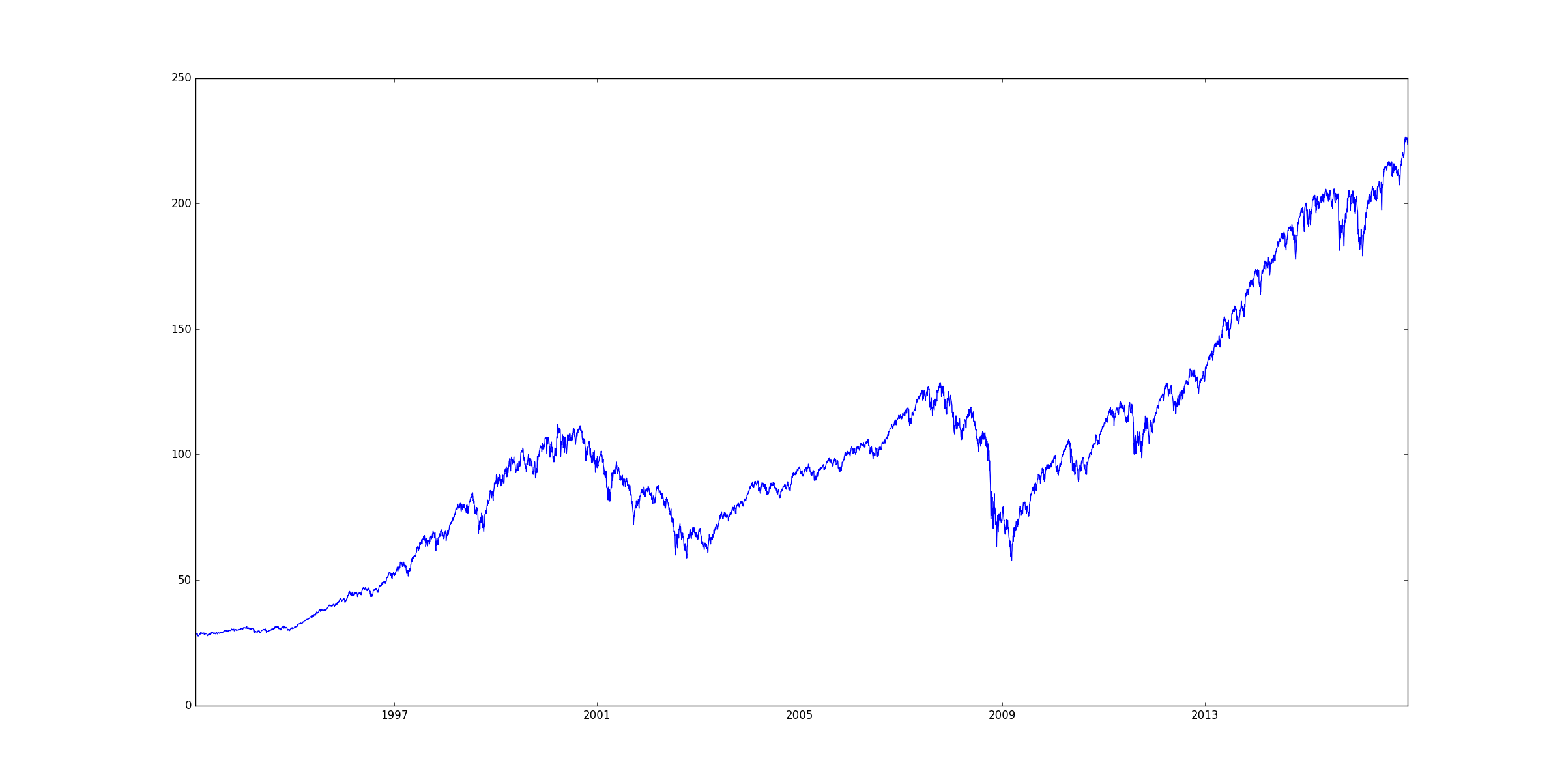
And a plot of the data:

When we calculate Hurst we get a value of roughly 0.436, which tells us that our series is moderately mean reverting.
# calculate Hurst
lag1 = 2
lags = range(lag1, 20)
tau = [sqrt(std(subtract(closes[lag:], closes[:-lag]))) for lag in lags]
plot(log(lags), log(tau)); show()
m = polyfit(log(lags), log(tau), 1)
hurst = m[0]*2
print 'hurst = ',hurst
Now, lets use the last 2000 values only.
# recent prices
closes_recent = spy['Adj Close'][-2000:]
plot(closes_recent); show()
# calculate Hurst of recent prices
lag1 = 2
lags = range(lag1, 20)
tau = [sqrt(std(subtract(closes_recent[lag:], closes_recent[:-lag]))) for lag in lags]
plot(log(lags), log(tau)); show()
m = polyfit(log(lags), log(tau), 1)
hurst = m[0]*2
print 'hurst = ',hurst
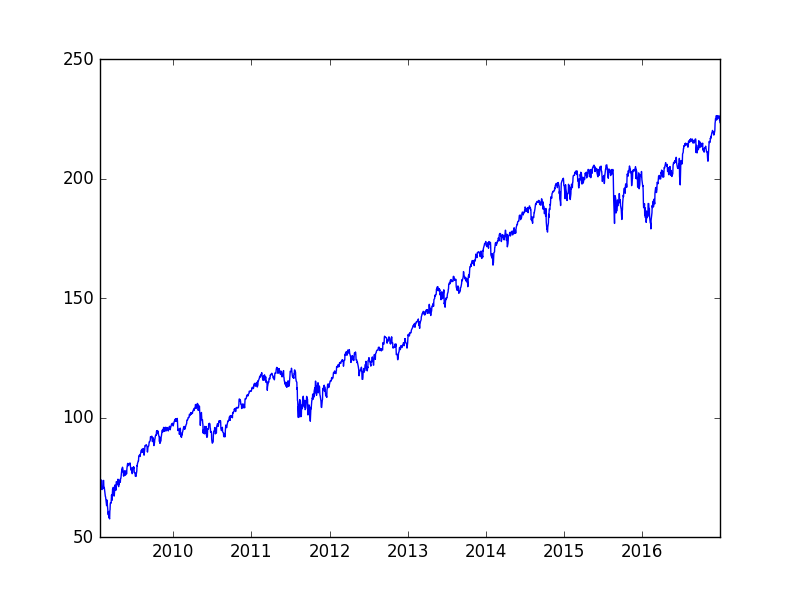
Here’s a plot of the recent SPY data:

We can see a clear trend so we would expect a Hurst value of greater than 0.5, however our algorithm returns H = 0.428, less than the value calculated for the longer period. This is clearly not in line with what we would expect, so let’s try looking at another range of lags. After trying a few different ranges, we found that using lags 300-400 resulted in a Hurst exponent of 0.668, which is more in line with what we would expect. However, if we plug those lags into the Hurst calculation for the entire series, we get H = 0.641, which may seem a little odd – at first glance anyway.
Impact of Lags on Hurst Calculation
We can draw a significant conclusion from these results: that the lags used to calculate Hurst have a much greater impact on the calculation than the particular segment of the time series analysed (for SPY, anyway). Further, when we look at the entire time series, we see that SPY is moderately mean-reverting for shorter lags. Lags up to about 20 are most mean reverting, and then H increases as we increase the lags used in its calculation. If we continue to increase the lags used to calculate H up to the range 300-400, we find that H indicates a moderately trending time series. We also find that for moderate lag values, H tends to approach 0.5, suggesting that SPY is also a random walk at some time scales.
SPY’s Mixed Mean-Reverting and Trending Behavior
This leads to the conclusion that SPY is neither absolutely mean reverting nor absolutely trending. Instead, Hurst indicates that it is moderately mean reverting over short time periods and tends to exhibit momentum over the longer term. I find this to be a pleasing result, one that is in line with the results of Jagadeesh and Titman (1993), who investigated momentum and found that multiple-month relative returns predict future returns. The result is also in line with what we tend to see over shorter time horizons in equities markets.
Consistency of Hurst Results Despite Visual Trends
What I find most extraordinary about these results is that they are consistent regardless of whether the time series appears to the naked eye to be trending (as in the sub-period from 2009 to the end of 2016) or mean reverting. Who could conclude, through observation of the price series alone, that the time series in Figure 2 was mean reverting over a short time horizon? I suppose if one looks closely, regular pullbacks in the uptrend are visible, but I don’t think it is obviously mean reverting. I believe that Hurst is therefore actually giving us some incredibly valuable insight into the behaviour of SPY.
Example: Random Walk with Uptrend
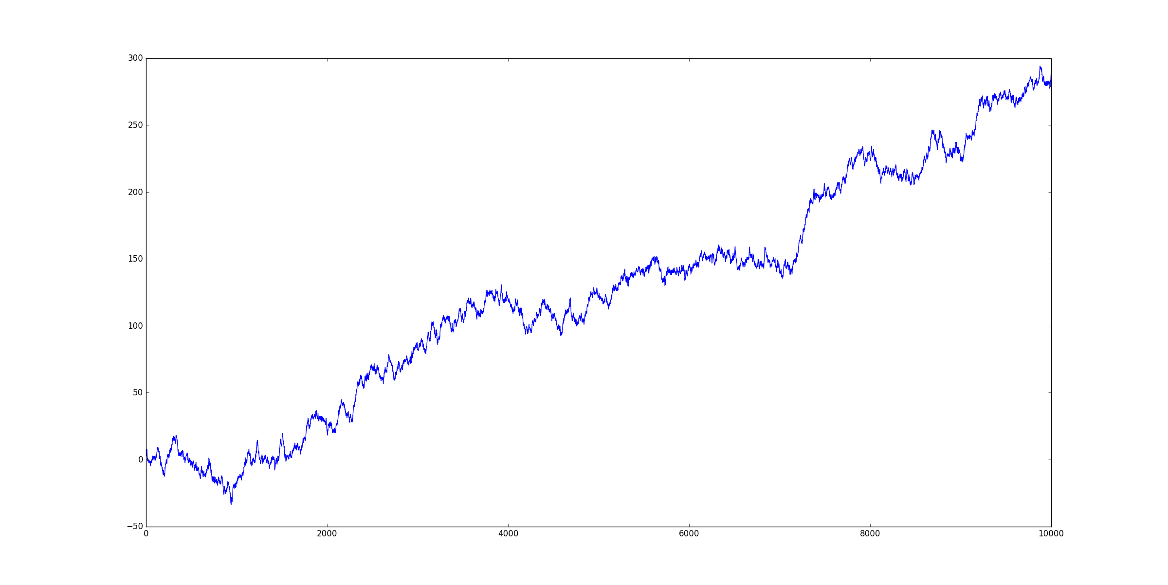
In order to see this effect more clearly, consider the following random walk, which by construction has no memory effect but does have a definite uptrend:
<pre class=”lang:python decode:true ” title=”Synthetic random walk with trend”># artifical random walk with trend rw = cumsum(randn(10000)+0.025) plot(rw)

Calculating Hurst for this series gives H = 0.502, which indeed corresponds to a random walk, despite the obvious uptrend. This is a great example of how our eyes can easily fail to detect the underlying dynamics of a time series.
Conclusions
In summary, I hope I have demonstrated that despite the attractive theory, utilising the Hurst calculation requires some deeper thought and analysis than simply plugging some numbers into an algorithm. However, if we take the time to investigate, we can obtain some potentially very useful insights.
Hurst is essentially a measure of the memory in a particular time series, and this memory can be both mean-reverting and trending at the same time, depending on the time scale.
In the case of the SPY ETF, the Hurst calculation showed that we would be more likely to trade successfully on short time frames if we utilised a mean-reversion trading model. Conversely, Hurst suggests that we would be more likely to be successful on longer time frames with momentum-style trading models.
We also saw that Hurst approaches 0.5
the random walk – for medium time frames, suggesting that we should perhaps avoid models that rely on that time horizon.
Of course, this assumes that the future will be like the past, which may or may not be the case. However, we did see some consistency in the H values calculated for the entire time series and a subset of that time series, which gives me some degree of confidence in this approach.
What do you think? How would you interpret the results I obtained for the SPY ETF? I would love to hear from you in the comments.


It would be interesting to test whether a hurst reading at a certain point in time is predictive for hurst readings in the future. If you’re looking for mean reversion systems and you find that the hurst exponent says 5 days is the optimal MR period for example, does this then hold for the future? Is the hurst exponent itself mean reverting over time or is it persistent?
Hey Matt, that’s a really good point and goes to the heart of why algo trading is so difficult – the analysis we perform holds for a certain period in the past but is not guaranteed to continue into the future. That is, the results of our analysis are non-stationary. What was interesting about the results I got on SPY was that the mean-reverting or trending behaviour of the time series (as indicated by Hurst) was actually quite consistent for various time scales when we sliced up the time series – even when the dominant regime looked completely different. What this means is that Hurst appears to be reasonably stationary when we keep the time scale constant, for SPY anyway. To me that’s a really surprising and significant result. I don’t know of too many other indicators or tests that show much consistency across obviously different overall regimes, and I guess you have found the same thing judging by your comment.
Interesting read. I find the conclusion that SPY seems to signal mean reverting behavior in short time periods and being stationary over time, to be consistent with my trading experience where I use weekly calendar spreads on underlyings like SPY, SPX, RUT, NDX.
It would be interesting to see if this also holds true for RUT, SPX, NDX. Is there code available in lite-C (Zorro) for the Hurst exponent?
Apologies if this is the wrong forum to ask a question such as this.
I was wondering if someone could help me understand where the sqrt and std come from in the following line of code that is used to calculate Hurst:
tau = [np.sqrt(np.std(np.subtract(ts[lag:], ts[:-lag]))) for lag in lags]
I believe it comes from the following principles (given on another RobotWealth page), but I just can’t reconcile how the formulae (copied below) lead to being able to use the code given, with the std and sqrt. I am also struggling to reconcile what the <| ….. |> symbols mean as well, am I right in thinking that the | | means absolute value or norm of a vector and as stated < … > means as average of all the data points?
I have seen this question pop up in 2 different forums, so I’m not the only person that is lost, but I’ve never seen it answered.
Thanks in advance and apologies if this question is not clear, I’m happy to provide further clarification, just let me know.
Formulae
Var(τ) = 〈|z(t + τ) − z(t)|^2〉
where
For a geometric random walk:
〈|z(t + τ) − z(t)|^2〉 ∼ τ
But if the series is either mean reverting or trending, this relationship will not hold, and instead we get
〈|z(t + τ) − z(t)|^2〉 ∼ τ^2H
This is a good question and worthy of more attention than I can devote to it presently. I will come back to this in due course though!
Many thanks for reading and posting, and apologies that I can’t respond in depth just yet.
Request: For loops are fairly inefficient for large datasets. This implementation of the tau function uses Python list comprehension. Is it more time efficient to implement the rescaled range (R/S) procedure using matrix operations?
statement tau = [sqrt(std(subtract(closes[lag:], closes[:-lag]))) for lag in lags] uses Python list comprehension.
https://python-reference.readthedocs.io/en/latest/docs/comprehensions/list_comprehension.html
closes is a “slice” from the spy dataframe which selects the column ‘Adj Close’. Adj Close is a closing price series for ticker symbol SPY.
closes = spy[‘Adj Close’][:]
https://pandas.pydata.org/docs/reference/api/pandas.DataFrame.html
The left [ and right ] are selectors using Python slice notation.
closes[lag:] selects from the row index lag to the end of the rows of the dataframe.
Rows are selected by counting from row index 0 (first row).
closes[:-lag] selects from the last row index -lag to the first row (row index 0) in the dataframe. Rows are selected in reverse order, counting from the last row in the dataframe.
The code snippet defines lags as a range of numbers from 2 to 20.
lag1 = 2
lags = range(lag1, 20)
for lag in lags is a Python for loop that iterates over the lags range.
order of operations: starting from the innermost parentheses first-
sqrt(std(subtract(closes[lag:], closes[:-lag])))
numpy function subtract, subtracts a vector closes[lag:] from vector closes[:-lag]
subtract(closes[lag:], closes[:-lag])
the standard deviation of the resulting vector is calculated:
std(subtract(closes[lag:], closes[:-lag]))
the square root of the standard deviation is calculated:
sqrt(std(subtract(closes[lag:], closes[:-lag])))
this sequence of vector selection, subtraction, calculating standard deviation, and the square root continues for each iteration from 2 to 20. this returns a list tau.
m = polyfit(log(lags), log(tau), 1)
m is the slope of the log-log plot. log(lags) and log(tau).
The hurst exponent is hurst = m[0]*2.
m[0] is the value of the list m at index 0.
hurst exponent is m[0] multiplied by 2.
Deriving the mathematical proof that this correctly implements the rescaled range (R/S) procedure would be an interesting puzzle to solve.
Here’s the wiki page on the rescaled range (R/S) procedure:
https://en.wikipedia.org/wiki/Hurst_exponent#Rescaled_range_(R/S)_analysis
Very cool, thanks for sharing!
Hi Kris, thank you so much for this article. Is any possible to get negative hurst exponent? I know the number should in the range of 0 and 1. But when I play with different lag, I got negative value. Is the problem of poly fit? how to solve that?
Thank you so much for any help.
thanks for the insightful post,
I never thought the lag parameters matters that much until this post, so thanks.
My query is what are your experience in running Hurst in different “time bars” , most of the examples I see on the internet are daily close price. Have anyone tried to run this on say like 5 minutes bar close price ? and does it tell you a different story ? and has anyone try running Hurst on a moving/sliding window ?
Thanks!
I am finding some inconsistencies here. First you mention that we have to look for other lags to accurately calculate Hurst exponent, because the value we were getting for 2-20 lags was not in line with our “expectations” based on what we see in the data:
“We can see a clear trend so we would expect a Hurst value of greater than 0.5, however our algorithm returns H = 0.428, less than the value calculated for the longer period. This is clearly not in line with what we would expect, so let’s try looking at another range of lags. After trying a few different ranges, we found that using lags 300-400 resulted in a Hurst exponent of 0.668, which is more in line with what we would expect.”
But then, towards the end you show the case of a generated random walk, where we see trends even though we later find (and already know) that the Hurst exponent is 0.5:
“Calculating Hurst for this series gives H = 0.502, which indeed corresponds to a random walk, despite the obvious uptrend. **This is a great example of how our eyes can easily fail to detect the underlying dynamics of a time series.**”
So, which is true? Can we take our intuition as a reliable guide to use the right lags to calculate the Hurst exponent, or we just keep calculating Hurst exponent over a wide range of lags and hope we find some convergence?
I don’t think either of those things is true, at least in any absolute sense.
Your question implies the existence of some “correct” value for Hurst. In the case where we know the underlying process that generated the data (as in the random walk example), we have an expected value of our Hurst exponent (0.5 in this case). Whether our estimate of Hurst gets close to that expected value is a function of sampling uncertainty.
The broader and more interesting point is that for the financial data series, for which we don’t know the generating process, we get different values for Hurst when we use different lags. This implies that we could estimate Hurst in different ways (using different lags for instance) to help us infer certain things about that unknown generating process. For example, we might be able to infer that over some historical time period, SPY tended to be noisily mean-reverting when sampled over lag A, and noisily trending when sampled over lag B. Of course, an even more interesting question is “do I expect that behaviour to persist in the future?”
It’s much more practical and interesting, from a trading perspective anyway, to think less in terms of “what’s the ‘correct’ value of some statistical parameter” (there isn’t one) and more in terms of “what does this observation tell me (and not tell me) about the thing I’m trying to understand.”