Part 3 of a series on Statistical Arbitrage for Independent Traders
Previously:
- A Tale of Two Prices (the core idea of stat arb)
- Moneyball (finding undervalued pairs using unconventional metrics)
In the last article, we built up a conceptual understanding of universe selection: how to find pairs that diverge and converge in a tradeable way. We talked about measuring the thing you actually care about directly, rather than reaching for statistical tests like cointegration that sound perfect but turn out to be unstable in practice.
The natural next step is to start trading them the traditional way. Long the cheap leg, short the expensive leg, wait for convergence, close.
I’ve been doing this for a few years now. And… it works. We’ve made money from it. But the simplicity comes at a cost. And the more I trade it this way, the more apparent it becomes that it leaves a lot on the table.
Limitations of traditional pairs trading
Let me describe what traditional pairs trading looks like in practice for the solo trader.
You’ve got your pair selection pipeline. It identifies, say, 100 pairs that score well on your metrics. Strong mean reversion characteristics, prices stay close together, same industry, liquid enough that you can trade them fairly easily, all the things you want.
But you can only trade a fraction of them.
In a regular portfolio margin account, a common structure for indie traders, pairs trading eats a lot of your buying power.
Each pair requires capital on both legs. If you’ve got $100k of buying power and you’re doing 10 pairs with equal weighting, that’s $10k per pair, $5k per leg. You’re basically maxed out.
If you try to trade more pairs by putting less on each leg, you start running into minimum commission fees and other frictions. The costs start to add up.
So you’ve got 100 good pairs. You trade 10 of them. What happens to the other 90?
Nothing.
All that signal, all that information from your really good selection process, essentially just sits there, hiding beneath the surface.

But there’s a deeper problem.
It’s not just that you can only trade a fraction of your universe. It’s that the capital you do deploy is being used inefficiently as well. Every time you put on a pair, you’re trading two legs. You’re using capital on both.
But typically, only one of those legs is actually mispriced.
Imagine you’ve got two oil stocks. One of them just had a random burst of selling. Some fund was liquidating a position, pushing the price down temporarily, so that the stock becomes cheap relative to the other.
That’s a pairs trade opportunity. You go long the cheap one, short the expensive one.
But look at what happened:
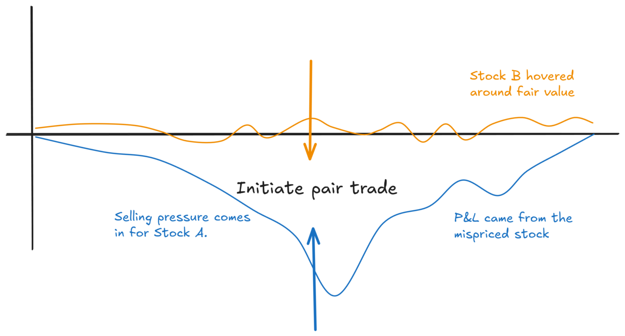
The cheap stock is mispriced. The other one was just sitting there at fair value the whole time. You traded both, but only one was actually doing the “work” of capturing the mispricing.
You’ve deployed capital on both legs, but the expected return is only coming from one of them.
That’s what I mean by capital inefficiency. You’re paying for two legs, but only getting the juice from one.
It gets worse when you think about transaction costs.
Every time you enter a pair, you cross the spread twice. You pay commissions twice. Every time you exit, same thing.
For a single directional trade, you’d pay one spread and one commission on entry, one on exit. For a pairs trade, you’re paying double.
And remember, the expected return is only coming from one leg. So your costs have doubled, but your expected return hasn’t.
Trade offs everywhere
Let’s go back to the 100 pairs problem.
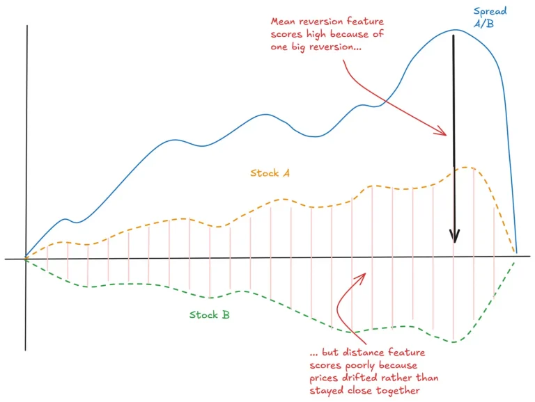
Say your pipeline identifies 100 pairs that look really good. Strong mean reversion, low distance metric, same industry, all the criteria we discussed last time.
If you could trade all 100 pairs, you’d have much more diversification. You’d be able to let the law of large numbers work for you. Individual pairs might go against you, but with enough of them, the statistics work out.
But you can’t trade 100 pairs. Capital constraints force you down to 10 or 20.
And here’s a subtle problem: those 100 pairs don’t involve 200 unique stocks. There’s a lot of overlap. Stock A might appear in five different pairs. Stock B might appear in eight.
All those pairs are telling you something about those individual stocks. Maybe Stock A appears as the cheap leg in five different pairs. That’s a pretty strong signal that Stock A is undervalued relative to its peers.
But in the traditional pairs approach, you can’t aggregate that information. You’re stuck trading pairs as isolated units. You can’t say, “Stock A looks cheap across lots of pairs, so I’ll just be long Stock A.”
Well, you could. But then you’d introduce a whole lot of variance, because you’d no longer be market neutral.
And that brings us to an important source of tension.
One reason people trade pairs in the first place is to be market neutral. You’re long one leg, short the other. General market moves don’t affect you (in theory). You’re just capturing the convergence.
If you only traded the mispriced leg, you’d have higher expected returns (lower costs), but much higher variance. You’re now net long or net short the market.
If the market moves against you, you could lose money even when you were right about the convergence:
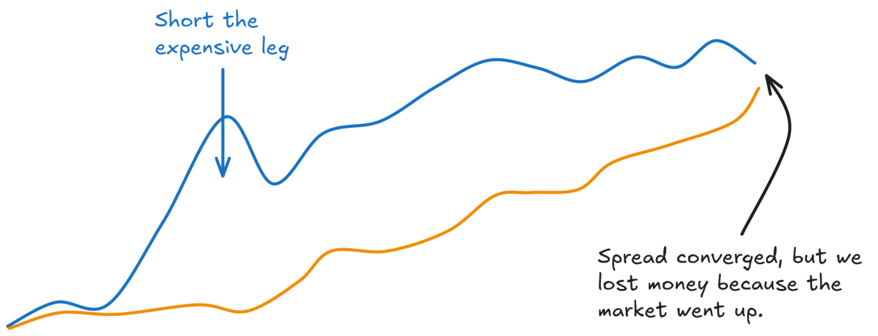
Equally, sometimes you’ll get lucky and make more than you expected to:
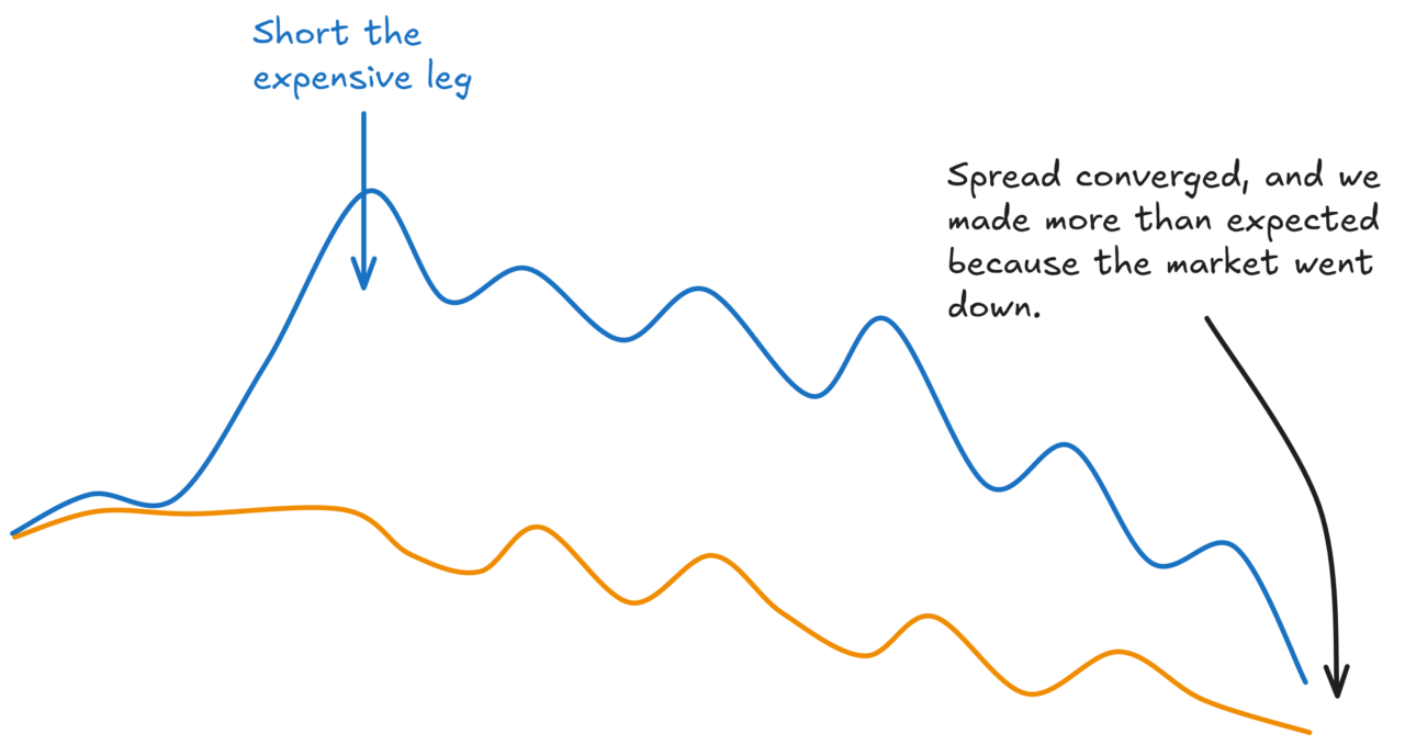
Over enough trades, you’d expect these to net off. But your P&L will be a lot more variable.
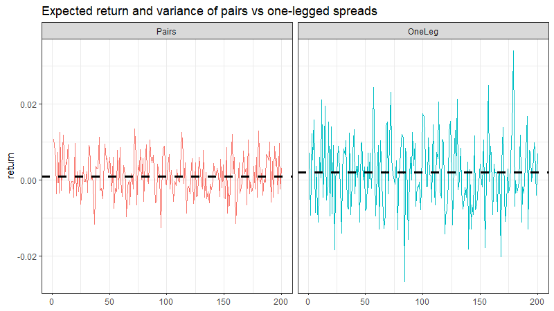
So you’ve got a tradeoff:
Traditional pairs: Lower variance (market neutral), but higher costs and capital inefficiency.
Just the mispriced leg: Higher expected returns (lower costs), but much higher variance.
How do you resolve this?
Well, you could just accept it and do the version that represents the best path through the trade-offs for you.
But we can do a little better…
More accurately, there might be another path through the trade-offs.
Perhaps we can trade some simplicity for the chance to have our delicious, higher expected return cake while eating less variance.
The high-frequency people do it by trading very fast. They’re not market neutral on each trade, but they turn over quickly enough that market moves net out before they notice the variance. The law of large numbers works in their favour through speed.
But that’s not realistic for most of us. We don’t have the infrastructure, the co-location, the data feeds. And even if we did, the edges at that speed are tiny and competitive.
For indie traders with slower strategies, we need a different approach.
The alternative is to go broad.
Instead of trading 10 pairs in isolation, you trade lots of individual positions, constructed intelligently so that market exposures tend to cancel out at the portfolio level.
You flatten your pair signals into signals on individual assets. You aggregate the information from many pairs. And you construct a portfolio that captures the juice while managing the risk.
And at the point you go from individual pairs to a portfolio, you open up the opportunity to add other signals to the mix, implement different risk models, and manage transaction costs more subtly.
If you’re really enthusiastic, you even infer things about a given stock from things that are happening throughout your broader network of flattened pairs.
This is what we might call a more “modern” statistical arbitrage approach. The general approach has been around for decades. And increasingly, it’s accessible to independent traders too.
Of course, there’s no free lunch.
You go from a super simple set of pairs that you could manage with a mouse and a TradingView subscription to something that you can easily get lost in if you’re not careful.
So it’s not something I’d recommend to every indie trader.
When trading is your part-time gig, there is immense value in simplicity. But if you’re a bit more ambitious about your trading, it’s something you might consider.
But it requires a shift in how you think about the problem. From pairs to portfolio. From isolated trades to system.
Remember in Part 1 when I said the divergence/convergence concept is simple? That core bet doesn’t change. What changes is how you express it.
Next time, we’ll dig into how that portfolio approach works, and why it solves (or at least reduces) the problems of higher variance, and signal and capital inefficiency.
Building the kind of infrastructure that supports a modern start arb approach yourself requires serious data engineering. Inside RW Pro, we’ve done the heavy lifting. But more on that another time.